

Operating Cisco Routers
INTERNOLD NETWORKS CCNA LIVE WEBCLASS (INCLW)
Operating Cisco Routers
Operating Cisco Routers
Getting an IPv4 network up and working requires some basic steps: installing routers, configuring their IPv4 addresses, optionally configuring some static IPv4 routes, and then configuring a routing protocol to dynamically learn routes. This chapter focuses on Step 1: how to install an enterprise-class Cisco router, with just enough configuration to get the router working, ready for those next steps.
This chapter breaks the topics into two major headings. The first discusses the physical installation of an enterprise-class Cisco router. The second section looks at the command-line interface (CLI) on a Cisco router, which has the same look and feel as the Cisco switch CLI. This section first lists the similarities between a switch and router CLI, and then introduces the configuration required to make the router start forwarding IP packets on its interfaces.
Installing Cisco Routers
Routers collectively provide the main feature of the network layer—the capability to forward packets end to end through a network. As introduced in Chapter 4, “Fundamentals of IPv4 Addressing and Routing,” routers forward packets by connecting to various physical network links, like Ethernet, serial links, and Frame Relay, and then using Layer 3 routing logic to choose where to forward each packet. As a reminder, Chapter 2, “Fundamentals of Ethernet LANs,” covered the details of making those physical connections to Ethernet networks, while Chapter 3, “Fundamentals of WANs,” covered the basics of cabling with WAN links.
This section examines some of the details of router installation and cabling, first from the enterprise perspective and then from the perspective of connecting a typical small office/home office (SOHO) to an ISP using high-speed Internet.
Installing Enterprise Routers
A typical enterprise network has a few centralized sites as well as lots of smaller remote sites. To support devices at each site (the computers, IP phones, printers, and other devices), the network includes at least one LAN switch at each site. In addition, each site has a router, which connects to the LAN switch and to some WAN link. The WAN link provides connectivity from each remote site, back to the central site, and to other sites through the connection to the central site.
Figures 17-1 and 17-2 show contrasting ways to draw parts of an enterprise network. Both show a typical branch office on the left, with a router and some end-user PCs. The central site, on the right, has basically the same components, plus some servers. The sites connect using a point-to-point serial link connecting the two routers. The first figure omits many of the cabling details, making the figure more useful when you want to discuss general Layer 3 concepts; the second figure shows the cabling details.

Generic Enterprise Network Diagram

More Detailed Cabling Diagram for the Same Enterprise Network
The Ethernet cables in Figure 17-2 should be familiar. In particular, routers use the same Ethernet cabling pinouts as PCs, so each router uses a UTP cable with a straight-through pinout.
Next, consider the hardware on the ends of the serial link, in particular where the channel service unit/data service unit (CSU/DSU) hardware resides on each end of the serial link. It sits either outside the router as a separate device (as shown on the left) or integrated into the router’s serial interface hardware (as shown on the right). Most new installations today include the CSU/DSU in the router’s serial interface.
Finally, the serial link requires some cabling inside the same wiring closet or other space between where the telco serial line terminates and where the router sits on a shelf or in a rack. The WAN cable installed by the telco typically has an RJ-48 connector, which is the same size and shape as an RJ-45 connector. The telco cable with the RJ-48 connector inserts into the CSU/DSU. In the example of Figure 17-2, at the central site, the telco cable connects directly into the router’s serial interface. At the branch office router, the cable connects to the external CSU/DSU, which then connects to the router serial interface using some other serial cable. (As a reminder, Chapter 3’s section “Leased-Line Cabling” introduced the basics of this cabling.)
Cisco Integrated Services Routers
Product vendors, including Cisco, typically provide several different types of router hardware. Today, routers often do much more work than simply routing packets—in fact, they serve as a device or platform from which to provide many network services. Cisco even brands their enterprise routers not just as routers, but as “integrated services routers,” emphasizing the multi-purpose nature of the products.
As an example, consider the networking functions needed at a typical branch office. A typical enterprise branch office needs a router for WAN/LAN connectivity, and a LAN switch to provide a high-performance local network and connectivity into the router and WAN. Many branches also need Voice over IP (VoIP) services to support IP phones, and several security services as well. Plus, it is hard to imagine a site with users that does not have Wi-Fi access today. So, rather than require multiple separate devices at one site, as shown in Figure 17-2, Cisco offers single devices that act as both router and switch, and provide other functions as well.
For the sake of learning and understanding the different functions, the CCENT and CCNA Routing and Switching exams focus on using a separate switch and separate router, which provides a much cleaner path for learning the basics.
Figure 17-3 shows a couple of pictures of the Cisco 4321 ISR, with some of the more important features highlighted. The top part of the figure shows a full view of the back of the router. This model comes with two built-in Gigabit Ethernet interfaces and two modular slots that allow you to add small cards called Network Interface Modules (NIMs). The bottom of the figure shows one example NIM (a NIM that provides two serial interfaces). The router has other items as well, including both an RJ-45 and USB console port.

Photos of a Model 4321 Cisco Integrated Services Router (ISR)
Physical Installation
Armed with the cabling details in figures like Figure 17-2, and the router hardware details in figures like Figure 17-3, you can physically install a router. To install a router, follow these steps:
Step 1. Connect any LAN cables to the LAN ports.
Step 2. If using an external CSU/DSU, connect the router’s serial interface to the CSU/DSU and the CSU/DSU to the line from the telco.
Step 3. If using an internal CSU/DSU, connect the router’s serial interface to the line from the telco.
Step 4. Connect the router’s console port to a PC (using a rollover cable), as needed, to configure the router.
Step 5. Connect a power cable from a power outlet to the power port on the router.
Step 6. Power on the router.
Note that the steps for router installation match those for a switch, except that Cisco enterprise routers typically have an on/off switch, while switches do not.
Installing Internet Access Routers
Routers play a key role in SOHO networks, connecting the LAN-attached end-user devices to a high-speed Internet access service. However, most SOHO products go by the name router, but happen to include many networking functions in a single device. Because of that, when learning about networking, it can be difficult to appreciate the different functions the device performs.
To help you understand the features of a router product used in a SOHO environment, Figure 17-4 first shows an example in which the SOHO network uses separate devices for each function. The first shows the devices and cabling, with a connection to the Internet using cable TV (CATV) as the high-speed Internet service.

Devices in a SOHO Network with High-Speed CATV Internet
This figure has many similarities to Figure 17-2, which shows a typical enterprise branch office. Some end-user PCs still connect with cabling to a switch, and the switch still connects to a router’s Ethernet interface. Other end-user devices use a wireless LAN, with a wireless access point, that also connects to the Ethernet LAN. For both the wired and wireless devices, the router still provides routing services, forwarding IP packets.
The main differences between the SOHO connection in Figure 17-4 and the enterprise branch in Figure 17-2 relate to the connection into the Internet. An Internet connection that uses CATV or digital subscriber line (DSL) needs a device that converts between the Layer 1 and 2 standards used on the CATV cable or DSL line and the Ethernet used by the router. These devices, commonly called cable modems and DSL modems, respectively, convert between CATV Layer 1 and Layer 2 standards to Ethernet, and vice versa. Similarly, DSL modems convert between the DSL signals over a home telephone line and Ethernet.
To physically install a SOHO network with the devices shown in Figure 17-4, you basically need the correct UTP cables for the Ethernet connections, and either the CATV cable (for cable Internet services) or a phone line (for DSL services). Note that the router used in Figure 17-4 simply needs to have two Ethernet interfaces—one to connect to the LAN switch and one to connect to the cable modem.
Today, most new SOHO installations use an integrated device rather than the separate devices shown in Figure 17-4. Consumer-grade devices are often called cable routers or DSL routers, while in fact they do all the functions shown in Figure 17-4, including the roles of
Router
Switch
Cable or DSL modem
Wireless access point
Hardware-enabled encryption
A newly installed high-speed SOHO Internet connection today probably looks more like Figure 17-5, with an integrated device.

SOHO Network, Using Cable Internet and an Integrated Device
Enabling IPv4 Support on Cisco Router Interfaces
Routers support a relatively large number of features, with a large number of configuration and EXEC commands to support those features. You will learn about many of these features throughout the rest of this book.
NOTE: For perspective, the Cisco router documentation includes a command reference, with an index to every single router command. A quick informal count of a recent IOS version listed around 5000 CLI commands.
This second section of the chapter focuses on commands related to router interfaces. To make routers work—that is, to route IPv4 packets—the interfaces must be configured. This section introduces the most common commands that configure interfaces, make them work, and give the interfaces IP addresses and masks.
Accessing the Router CLI
Accessing a router’s command-line interface (CLI) works much like a switch. In fact, it works so much like accessing a Cisco switch CLI that this book relies on Chapter 6, “Using the Command-Line Interface,” instead of repeating the same details here. If the details from Chapter 6 are not fresh in your memory, it might be worthwhile to spend a few minutes briefly reviewing Chapter 6 as well as Chapter 9, “Configuring Switch Interfaces,” before reading further.
Cisco switches and routers share many of the same CLI navigation features, and many of the same configuration commands for management features. The following list mentions the highlights:
User and Enable (privileged) mode
Entering and exiting configuration mode, using the configure terminal, end, and exit commands and the Ctrl+Z key sequence
Configuration of console, Telnet (vty), and enable secret passwords
Configuration of Secure Shell (SSH) encryption keys and username/password login credentials
Configuration of the hostname and interface description
Configuration of Ethernet interfaces that can negotiate speed using the speed and duplex commands
Configuration of an interface to be administratively disabled (shutdown) and administratively enabled (no shutdown)
Navigation through different configuration mode contexts using commands like line console 0 and interface type number
CLI help, command editing, and command recall features
The meaning and use of the startup-config (in NVRAM), running-config (in RAM), and external servers (like TFTP), along with how to use the copy command to copy the configuration files and IOS images
At first glance, this list seems to cover most everything covered in Chapter 8—and it does cover most of the details; however, a couple of topics covered in Chapter 8 do work differently with the router CLI as compared to the switch CLI, as follows:
The configuration of IP addresses differs in some ways, with switches using a VLAN interface and routers using an IP address configured on each working interface.
Many Cisco router models have an auxiliary (Aux) port, intended to be connected to an external modem and phone line to allow remote users to dial in to the router, and access the CLI, by making a phone call. Cisco switches do not have auxiliary ports.
Router IOS defaults to disallow both Telnet and SSH into the router because of the default setting of transport input none in vty configuration mode. Chapter 8, “Configuring Basic Switch Management,” already discussed the various options on this command to enable Telnet (transport input telnet), SSH (transport input ssh), or both (transport input all or transport input telnet ssh).
The router CLI also differs from a switch CLI just because switches and routers do different things. For example, Cisco Layer 2 switches support the show mac address-table command, but these Layer 2–only devices do not support the show ip route command, which routers use to list IPv4 routes. Some Cisco routers can do IP routing but not Layer 2 switching, so they support the show ip route command but not the show mac address-table command.
NOTE: The book includes a video that shows how to navigate the router CLI; you can find this video on the DVD and on the companion website.
Router Interfaces
One minor difference between Cisco switches and routers is that routers support a much wider variety of interfaces. Today, LAN switches support Ethernet LAN interfaces of various speeds. Routers support a variety of other types of interfaces, including serial interfaces, cable TV, DSL, 3G/4G wireless, and others not mentioned in this book.
Most Cisco routers have at least one Ethernet interface of some type. Many of those Ethernet interfaces support multiple speeds and use autonegotiation, so for consistency, the router IOS refers to these interfaces based on the fastest speed. For example, a 10-Mbps-only Ethernet interface would be configured with the interface ethernet number configuration command, a 10/100 interface with the interface fastethernet number command, and a 10/100/1000 interface with the interface gigabitethernet number command.
Some Cisco routers have serial interfaces. As you might recall from Chapter 3, Cisco routers use serial interfaces to connect to a serial link. Each point-to-point serial link can then use High-Level Data Link Control (HDLC, the default) or Point-to-Point Protocol (PPP).
Routers refer to interfaces in many commands, first by the type of interface (Ethernet, Fast Ethernet, Serial, and so on) and then with a unique number of that router. On routers, the interface numbers might be a single number, two numbers separated by a slash, or three numbers separated by slashes. For example, all three of the following configuration commands are correct on at least one model of Cisco router:
interface ethernet 0
interface fastEthernet 0/1
interface gigabitethernet 0/0
interface serial 1/0/1
Two of the most common commands to display the interfaces, and their status, are the show ip interface brief and show interfaces commands. The first of these commands displays a list with one line per interface, with some basic information, including the interface IP address and interface status. The second command lists the interfaces, but with a large amount of information per interface. Example 17-1 shows a sample of each command.
Example 17-1 Listing the Interfaces in a Router

Listing the Interfaces in a Router
NOTE: Commands that refer to router interfaces can be significantly shortened by truncating the words. For example, sh int fa0/0 can be used instead of show interfaces fastethernet 0/0. In fact, many network engineers, when looking over someone’s shoulder, would say something like “just do a show int F-A-oh-oh command” in this case, rather than speaking the long version of the command.
Also, note that the show interfaces command lists a text interface description on about the third line, if configured. In this case, interface S0/0/0 had been previously configured with the description Link in lab to R2’s S0/0/1 command in interface configuration mode for interface S0/0/0. The description interface subcommand provides an easy way to keep small notes about what router interfaces connect to which neighboring devices, with the show interfaces command listing that information.
Interface Status Codes
Each interface has two interface status codes. To be usable, the two interface status codes must be in an “up” state. The first status code refers essentially to whether Layer 1 is working, and the second status code mainly (but not always) refers to whether the data link layer protocol is working. Table 17-2 summarizes these two status codes.

Interface Status Codes and Their Meanings
Several combinations of interface status codes exist, as summarized in Table 17-3. The table lists the status codes in order, from being disabled on purpose by the configuration to a fully working state.
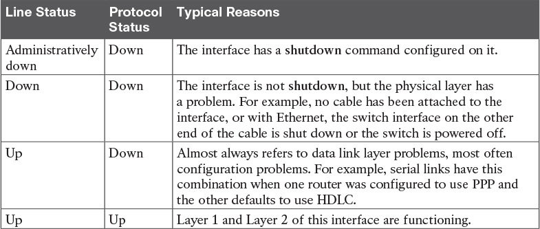
Typical Combinations of Interface Status Codes
For some examples, look back at Example 17-1’s show ip interface brief command, to the three interfaces in the following list. The interfaces in this list each have a different combination of interface status codes; the list details the specific reasons for this status code in the lab used to create this example for the book.
G0/0: The interface is down/down, in this case because no cable was connected to the interface.
G0/1: The interface is administratively down/down, because the configuration includes the shutdown command under the G0/1 interface.
S0/0/0: The interface is up/up because a serial cable is installed, connected to another router in a lab, and is working.
Router Interface IP Addresses
Cisco enterprise routers require at least some configuration beyond the default configuration before they will do their primary job: routing IP packets. The following facts tell us that to make a router ready to route IPv4 packets on an interface, you need to enable the interface and assign it an IPv4 address:
Most Cisco router interfaces default to a disabled (shutdown) state and should be enabled with the no shutdown interface subcommand.
Cisco routers do not route IP packets in or out an interface until an IP address and mask have been configured; by default, no interfaces have an IP address and mask.
Cisco routers attempt to route IP packets for any interfaces that are in an up/up state and that have an IP address/mask assigned.
To configure the address and mask, simply use the ip address address mask interface subcommand. Figure 17-6 shows a simple IPv4 network, the same network used in several of the subnetting examples in Part IV of this book. The figure shows the IPv4 addresses on Router R1, with Example 17-2 showing the matching configuration.

IPv4 Addresses Used in Example 17-2
Example 17-2 Configuring IP Addresses on Cisco Routers
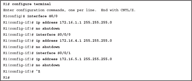
Configuring IP Addresses on Cisco Routers
Example 17-3 shows the output of the show protocols command. This command confirms the state of each of the three R1 interfaces in Figure 17-6 and the IP address and mask configured on those same interfaces.
Example 17-3 Verifying IP Addresses on Cisco Routers
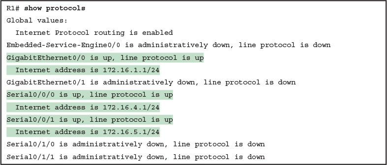
Verifying IP Addresses on Cisco Routers
One of the first actions to take when verifying whether a router is working is to find the interfaces, check the interface status, and check to see whether the correct IP addresses and masks are used. Examples 17-1 and 17-3 showed samples of the key show commands, while Table 17-4 summarizes those commands and the types of information they display.

Key Commands to List Router Interface Status
Bandwidth and Clock Rate on Serial Interfaces
Cisco happens to place more of the WAN technologies in the ICND2 half of CCNA Routing and Switching exam content; however, you also need to be able to practice router configurations for ICND1 exam preparation, which could include using serial interfaces on any routers you buy or borrow for your lab. If you decide to build your own study lab with real gear, you need to know just a little more information about serial links. This last topic in the chapter discusses those details.
As mentioned back in Chapter 3, WAN serial links can run at a wide variety of speeds. To deal with the wide range of speeds, routers physically slave themselves to the speed as dictated by the CSU/DSU through a process called clocking. As a result, routers can use serial links without the need for additional configuration or autonegotiation to sense the serial link’s speed. The CSU/DSU knows the speed, the CSU/DSU sends clock pulses over the cable to the router, and the router reacts to the clocking signal.
To build a serial link in a home lab, the routers can use serial interface cards that normally use an external CSU/DSU, and make a serial link, without requiring the expense of two CSU/DSUs. Chapter 3’s Figure 3-5 introduced this concept, and it is repeated here as Figure 17-7. To make it work, the link uses two serial cables—one a DTE cable and the other a DCE cable—which swap the transmit and receive pair on the cables.
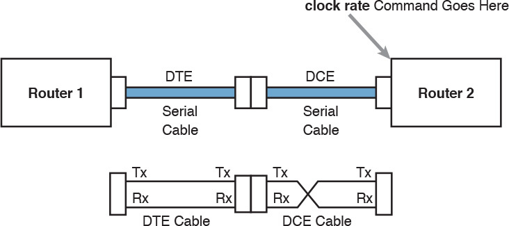
Serial Link in Lab
Using the correct cabling works, as long as you add one command: the clock rate interface subcommand. This command tells that router the speed at which to transmit bits on a serial link like the one shown in Figure 17-7. The clock rate command is not needed on real serial links, because the CSU/DSU provides the clocking. When you create a serial link in the lab using cables, without any real CSU/DSUs on the link, the router with the DCE cable must supply that clocking function, and the clock rate command tells the router to provide it.
NOTE: Newer router IOS versions automatically add a default clock rate 2000000 command on serial interfaces that have a DCE cable connected to them. While helpful, this speed might be too high for some types of back-to-back serial cables, so consider using a lower speed in lab.
Example 17-4 shows the configuration of the clock rate command using the same Router R1 used in the earlier Example 17-2. The end of the example verifies that this router can use the clock rate command with the show controllers command. This command confirms that R1 has a V.35 DCE cable connected.
Example 17-4 Router R1 Configuration with the clock rate Command

Router R1 Configuration with the clock rate Command
NOTE: The clock rate command does not allow just any speed to be configured. However, the list of speeds does vary from router to router.
Some people confuse the router bandwidth command with the clock rate command. The clock rate command sets the actual Layer 1 speed used on the link, if no CSU/DSU is used, as just described. Conversely, every router interface has a bandwidth setting, either by default or configured. The bandwidth of the interface is the documented speed of the interface, which does not have to match the actual Layer 1 speed used on the interface.
That bandwidth setting does not impact how fast the interface transmits data. Instead, routers use the interface bandwidth setting as both documentation and as input to some other processes. For instance, the Open Shortest Path First (OSPF) and Enhanced Interior Gateway Routing Protocol (EIGRP) routing protocols, discussed in the ICND2 part of the CCNA Routing and Switching material, base their routing protocol metrics on the bandwidth by default.
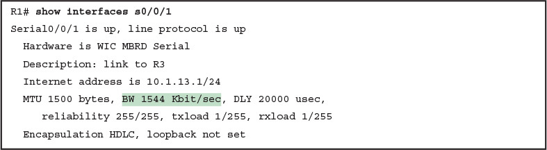
Example 17-5 highlights the bandwidth setting on Router R1’s S0/0/1 interface, as configured in the previous example. In that previous example, the clock rate 128000 command sets the clock rate to 128 kbps, but it leaves the bandwidth command unset. As a result, IOS uses the default serial bandwidth setting of 1544, which means 1544 kbps—which is the speed of a T1 serial link.
Example 17-5 Router Bandwidth Settings
Router Bandwidth Settings
The common mistake people make is to know about clock rate, but mistakenly think that the bandwidth setting is just another term for “clock rate.” It is not. Follow these rules to find these two interface settings:
To see the clock rate, look for the clock rate interface subcommand in the configuration, or use the show controllers serial type number command (as shown in Example 17-4.)
To see the bandwidth setting on an interface, look for the bandwidth interface subcommand in the configuration, or use the show interfaces [type number] command (as shown in Example 17-5).
Note that using default bandwidth settings on most router interfaces makes sense, with the exception of serial interfaces. IOS defaults to a bandwidth of 1544 (meaning 1544 kbps, or 1.544 Mbps) for serial interfaces, regardless of the speed dictated by the provider or by a clock rate command in the lab. Most engineers set the bandwidth to match the actual speed, for example, using the bandwidth 128 interface subcommand on a link running at 128 kbps. On Ethernet 10/100 or 10/100/1000 interfaces, the router knows the speed used, and dynamically sets the Ethernet interface’s bandwidth to match.
Router Auxiliary Port
Both routers and switches have a console port to allow administrative access, but most Cisco routers have an extra physical port called an auxiliary (Aux) port. The Aux port typically serves as a means to make a phone call to connect into the router to issue commands from the CLI.
The Aux port works like the console port, except that the Aux port is typically connected through a cable to an external analog modem, which in turn connects to a phone line. Then, the engineer uses a PC, terminal emulator, and modem to call the remote router. After being connected, the engineer can use the terminal emulator to access the router CLI, starting in user mode as usual.
Aux ports can be configured beginning with the line aux 0 command to reach aux line configuration mode. From there, all the commands for the console line, covered mostly in Chapter 8, “Configuring Basic Switch Management,” can be used. For example, the login and password password subcommands on the aux line could be used to set up simple password checking when a user dials in.

Analyzing Existing Subnets
INTERNOLD NETWORKS CCNA LIVE WEBCLASS (INCLW)
Analyzing Existing Subnets
Contents
Analyzing Existing Subnets
Often, a networking task begins with the discovery of the IP address and mask used by some host. Then, to understand how the internetwork routes packets to that host, you must find key pieces of information about the subnet, specifically the following:
- Subnet ID
- Subnet broadcast address
- Subnet’s range of usable unicast IP addresses
This lesson discusses the concepts and math to take a known IP address and mask, and then fully describe a subnet by finding the values in this list. These specific tasks might well be the most important IP skills in the entire IP addressing and subnetting topics in this course, because these tasks might be the most commonly used tasks when operating and troubleshooting real networks.
Defining a Subnet
An IP subnet is a subset of a classful network, created by choice of some network engineer. However, that engineer cannot pick just any arbitrary subset of addresses; instead, the engineer must follow certain rules, such as the following:
- The subnet contains a set of consecutive numbers.
- The subnet holds 2H numbers, where H is the number of host bits defined by the subnet mask.
- Two special numbers in the range cannot be used as IP addresses:
- The first (lowest) number acts as an identifier for the subnet (subnet ID).
- The last (highest) number acts as a subnet broadcast address.
- The remaining addresses, whose values sit between the subnet ID and subnet broadcast address, are used as unicast IP addresses.
This section reviews and expands the basic concepts of the subnet ID, subnet broadcast address, and range of addresses in a subnet.
An Example with Network 172.16.0.0 and Four Subnets
Imagine that you work at the customer support center, where you receive all initial calls from users who have problems with their computer. You coach the user through finding her IP address and mask: 172.16.150.41, mask 255.255.192.0. One of the first and most common tasks you will do based on that information is to find the subnet ID of the subnet in which that address resides. (In fact, this subnet ID is sometimes called the resident subnet, because the IP address exists in or resides in that subnet.)
Before getting into the math, examine the mask (255.255.192.0) and classful network (172.16.0.0) for a moment. From the mask you can find the structure of the addresses in the subnet, including the number of host and subnet bits. That analysis tells you that two subnet bits exist, meaning that there should be four (22) subnets. Figure 1 shows the idea.

Figure 1: Address Structure: Class B Network, /18 Mask
NOTE: This lesson, like the others in this part of the course, assumes that one mask is used throughout an entire classful network.
Because each subnet uses a single mask, all subnets of this single IP network must be the same size, because all subnets have the same structure. In this example, all four subnets will have the structure shown in the figure, so all four subnets will have 214 – 2 host addresses.
Next, consider the big picture of what happens with this example subnet design: The one Class B network now has four subnets of equal size. Conceptually, if you represent the entire Class B network as a number line, each subnet consumes one-fourth of the number line, as shown in Figure 2. Each subnet has a subnet ID—the numerically lowest number in the subnet—so it sits on the left of the subnet. And each subnet has a subnet broadcast address—the numerically highest number in the subnet—so it sits on the right side of the subnet.

Figure 2: Network 172.16.0.0, Divided into Four Equal Subnets
The rest of this lesson focuses on how to take one IP address and mask and discover the details about that one subnet in which the address resides. In other words, you see how to find the resident subnet of an IP address. Again, using IP address 172.16.150.41 and mask 255.255.192.0 as an example, Figure 3 shows the resident subnet, along with the subnet ID and subnet broadcast address that bracket the subnet.

Figure 3: Resident Subnet for 172.16.150.41, 255.255.192.0
Subnet ID Concepts
A subnet ID is simply a number used to succinctly represent a subnet. When listed along with its matching subnet mask, the subnet ID identifies the subnet and can be used to derive the subnet broadcast address and range of addresses in the subnet. Rather than having to write down all these details about a subnet, you simply need to write down the subnet ID and mask, and you have enough information to fully describe the subnet.
The subnet ID appears in many places, but it is seen most often in IP routing tables. For example, when an engineer configures a router with its IP address and mask, the router calculates the subnet ID and puts a route into its routing table for that subnet. The router typically then advertises the subnet ID/mask combination to neighboring routers with some IP routing protocol. Eventually, all the routers in an enterprise learn about the subnet—again using the subnet ID and subnet mask combination—and display it in their routing tables. (You can display the contents of a router’s IP routing table using the show ip route command.)
Unfortunately, the terminology related to subnets can sometimes cause problems. First, the terms subnet ID, subnet number, and subnet address are synonyms. In addition, people sometimes simply say subnet when referring to both the idea of a subnet and the number that is used as the subnet ID. When talking about routing, people sometimes use the term prefix instead of subnet. The term prefix refers to the same idea as subnet; it just uses terminology from the classless addressing way to describe IP addresses.
The biggest terminology confusion arises between the terms network and subnet. In the real world, people often use these terms synonymously, and that is perfectly reasonable in some cases. In other cases, the specific meaning of these terms, and their differences, matter to what is being discussed.
For example, people often might say, “What is the network ID?” when they really want to know the subnet ID. In another case, they might want to know the Class A, B, or C network ID. So, when one engineer asks something like, “What’s the net ID for 172.16.150.41 slash 18?” use the context to figure out whether he wants the literal classful network ID (172.16.0.0, in this case) or the literal subnet ID (172.16.128.0, in this case).
For the exams, be ready to notice when the terms subnet and network are used, and then use the context to figure out the specific meaning of the term in that case.
Table 2 summarizes the key facts about the subnet ID, along with the possible synonyms, for easier review and study.

Table 2 Summary of Subnet ID Key Facts
Subnet Broadcast Address
The subnet broadcast address has two main roles: to be used as a destination IP address for the purpose of sending packets to all hosts in the subnet, and as a means to find the high end of the range of addresses in a subnet.
The original purpose for the subnet broadcast address was to give hosts a way to send one packet to all hosts in a subnet, and to do so efficiently. For example, a host in subnet A could send a packet with a destination address of subnet B’s subnet broadcast address. The routers would forward this one packet just like a packet sent to a host in subnet B. After the packet arrives at the router connected to subnet B, that last router would then forward the packet to all hosts in subnet B, typically by encapsulating the packet in a data link layer broadcast frame. As a result, all hosts in host B’s subnet would receive a copy of the packet.
The subnet broadcast address also helps you find the range of addresses in a subnet, because the broadcast address is the last (highest) number in a subnet’s range of addresses. To find the low end of the range, calculate the subnet ID; to find the high end of the range, calculate the subnet broadcast address.
Table 3 summarizes the key facts about the subnet broadcast address, along with the possible synonyms, for easier review and study.

Table 3 Summary of Subnet Broadcast Address Key Facts
Range of Usable Addresses
The engineers implementing an IP internetwork need to know the range of unicast IP addresses in each subnet. Before you can plan which addresses to use as statically assigned IP addresses, which to configure to be leased by the DHCP server, and which to reserve for later use, you need to know the range of usable addresses.
To find the range of usable IP addresses in a subnet, first find the subnet ID and the subnet broadcast address. Then, just add 1 to the fourth octet of the subnet ID to get the first (lowest) usable address, and subtract 1 from the fourth octet of the subnet broadcast address to get the last (highest) usable address in the subnet.
For example, Figure 3 showed subnet ID 172.16.128.0, mask /18. The first usable address is simply one more than the subnet ID (in this case, 172.16.128.1). That same figure showed a subnet broadcast address of 172.16.191.255, so the last usable address is one less, or 172.16.191.254.
Now that this section has described the concepts behind the numbers that collectively define a subnet, the rest of this lesson focuses on the math used to find these values.
Analyzing Existing Subnets: Binary
What does it mean to “analyze a subnet”? For this course, it means that you should be able to start with an IP address and mask and then define key facts about the subnet in which that address resides. Specifically, that means discovering the subnet ID, subnet broadcast address, and range of addresses. The analysis can also include the calculation of the number of addresses in the subnet but this lesson does not review those concepts.
Many methods exist to calculate the details about a subnet based on the address/mask. This section begins by discussing some calculations that use binary math, with the next section showing alternatives that use only decimal math. Although many people prefer the decimal method for going fast on the exams, the binary calculations ultimately give you a better understanding of IPv4 addressing. In particular, if you plan to move on to attain Cisco certifications beyond CCNA Routing and Switching, you should take the time to understand the binary methods discussed in this section, even if you use the decimal methods for the exams.
Finding the Subnet ID: Binary
To start this section that uses binary, first consider a simple decimal math problem. The problem: Find the smallest three-digit decimal number that begins with 4. The answer, of course, is 400. And although most people would not have to break down the logic into steps, you know that 0 is the lowest-value digit you can use for any digit in a decimal number. You know that the first digit must be a 4, and the number is a three-digit number, so you just use the lowest value (0) for the last two digits, and find the answer: 400.
This same concept, applied to binary IP addresses, gives you the subnet ID. You have seen all the related concepts in other lessons, so if you already intuitively know how to find the subnet ID in binary, great! If not, the following key facts should help you see the logic:
All numbers in the subnet (subnet ID, subnet broadcast address, and all usable IP addresses) have the same value in the prefix part of the numbers.
The subnet ID is the lowest numeric value in the subnet, so its host part, in binary, is all 0s.
To find the subnet ID in binary, you take the IP address in binary and change all host bits to binary 0. To do so, you need to convert the IP address to binary. You also need to identify the prefix and host bits, which can be easily done by converting the mask (as needed) to prefix format. Figure 4 shows the idea, using the same address/mask as in the earlier examples in this lesson: 172.16.150.41, mask /18.

Figure 4: Binary Concept: Convert the IP Address to the Subnet ID
Starting at the top of Figure 4, the format of the IP address is represented with 18 prefix (P) and 14 host (H) bits in the mask (Step 1). The second row (Step 2) shows the binary version of the IP address, converted from the dotted-decimal notation (DDN) value 172.16.150.41. (If you have not yet used the conversion table in Appendix A, it might be useful to double-check the conversion of all four octets based on the table.)
The next two steps show the action to copy the IP address’s prefix bits (Step 3) and give the host bits a value of binary 0 (Step 4). This resulting number is the subnet ID (in binary).
The last step, not shown in Figure 4, is to convert the subnet ID from binary to decimal. This course shows that conversion as a separate step, in Figure 5, mainly because many people make a mistake at this step in the process. When converting a 32-bit number (like an IP address or IP subnet ID) back to an IPv4 DDN, you must follow this rule:
Convert 8 bits at a time from binary to decimal, regardless of the line between the prefix and host parts of the number.

Figure 5: Converting the Subnet ID from Binary to DD
Figure 5 shows this final step. Note that the third octet (the third set of 8 bits) has 2 bits in the prefix and 6 bits in the host part of the number, but the conversion occurs for all 8 bits.
NOTE: To convert from DDN to binary, for each octet, find the decimal value in the table and then write down the 8-bit binary equivalent. To convert from binary back to DDN, for each octet of 8 bits, find the matching binary entry in the table and write down the corresponding decimal value. For example, 172 converts to binary 10101100, and 00010000 converts to decimal 16.
Finding the Subnet Broadcast Address: Binary
Finding the subnet broadcast address uses a similar process. To find the subnet broadcast address, use the same binary process used to find the subnet ID, but instead of setting all the host bits to the lowest value (all binary 0s), set the host part to the highest value (all binary 1s). Figure 6 shows the concept.
Figure 6: Finding a Subnet Broadcast Address: Binary
The process in Figure 6 demonstrates the same first three steps shown in Figure 4. Specifically, it shows the identification of the prefix and host bits (Step 1), the results of converting the IP address 172.16.150.41 to binary (Step 2), and the copying of the prefix bits (first 18 bits, in this case). The difference occurs in the host bits on the right, changing all host bits (the last 14, in this case) to the largest possible value (all binary 1s). The final step converts the 32-bit subnet broadcast address to DDN format. Also, remember that with any conversion from DDN to binary or vice versa, the process always converts using 8 bits at a time. In particular, in this case, the entire third octet of binary 10111111 is converted back to decimal 191.
Binary Practice Problems
Figures 4 and 5 demonstrate a process to find the subnet ID using binary math. The following process summarizes those steps in written form for easier reference and practice:
- Step 1. Convert the mask to prefix format to find the length of the prefix (/P) and the length of the host part (32 – P).
- Step 2. Convert the IP address to its 32-bit binary equivalent.
- Step 3. Copy the prefix bits of the IP address.
- Step 4. Write down 0s for the host bits.
- Step 5. Convert the resulting 32-bit number, 8 bits at a time, back to decimal.
The process to find the subnet broadcast address is exactly the same, except in Step 4, you set the bits to 1s, as shown in Figure 6.
Take a few moments and run through the following five practice problems on scratch paper. In each case, find both the subnet ID and subnet broadcast address. Also, record the prefix style mask:
- 1. 8.1.4.5, 255.255.0.0
- 2. 130.4.102.1, 255.255.255.0
- 3. 199.1.1.100, 255.255.255.0
- 4. 130.4.102.1, 255.255.252.0
- 5. 199.1.1.100, 255.255.255.224
Tables 4 through 8 show the results for the five different examples. The tables show the host bits in bold, and they include the binary version of the address and mask and the binary version of the subnet ID and subnet broadcast address.

Table 4 Subnet Analysis for Subnet with Address 8.1.4.5, Mask 255.255.0.0

Table 5 Subnet Analysis for Subnet with Address 130.4.102.1, Mask 255.255.255.0

Table 6 Subnet Analysis for Subnet with Address 199.1.1.100, Mask 255.255.255.0

Table 7 Subnet Analysis for Subnet with Address 130.4.102.1, Mask 255.255.252.0

Table 8 Subnet Analysis for Subnet with Address 199.1.1.100, Mask 255.255.255.224
Shortcut for the Binary Process
The binary process described in this section so far requires that all four octets be converted to binary and then back to decimal. However, you can easily predict the results in at least three of the four octets, based on the DDN mask. You can then avoid the binary math in all but one octet and reduce the number of binary conversions you need to do.
First, consider an octet, and that octet only, whose DDN mask value is 255. The mask value of 255 converts to binary 11111111, which means that all 8 bits are prefix bits. Thinking through the steps in the process, at Step 2, you convert the address to some number. At Step 3, you copy the number. At Step 4, you convert the same 8-bit number back to decimal. All you did in those three steps, in this one octet, is convert from decimal to binary and convert the same number back to the same decimal value!
In short, the subnet ID (and subnet broadcast address) are equal to the IP address in octets for which the mask is 255.
For example, the resident subnet ID for 172.16.150.41, mask 255.255.192.0 is 172.16.128.0. The first two mask octets are 255. Rather than think about the binary math, you could just start by copying the address’s value in those two octets: 172.16.
Another shortcut exists for octets whose DDN mask value is decimal 0, or binary 00000000. With a decimal mask value of 0, the math always results in a decimal 0 for the subnet ID, no matter the beginning value in the IP address. Specifically, just look at Steps 4 and 5 in this case: At Step 4, you would write down 8 binary 0s, and at Step 5, convert 00000000 back to decimal 0.
The following revised process steps take these two shortcuts into account. However, when the mask is neither 0 nor 255, the process requires the same conversions. At most, you have to do only one octet of the conversions. To find the subnet ID, apply the logic in these steps for each of the four octets:
- Step 1. If the mask = 255, copy the decimal IP address for that octet.
- Step 2. If the mask = 0, write down a decimal 0 for that octet.
- Step 3. If the mask is neither 0 nor 255 in this octet, use the same binary logic as shown in the section “Finding the Subnet ID: Binary,” earlier in this lesson.
Figure 7 shows an example of this process, again using 172.16.150.41, 255.255.192.0.

Figure 7 Binary Shortcut Example
To find the subnet broadcast address, you can use a decimal shortcut similar to the one used to find the subnet ID: For DDN mask octets equal to decimal 0, set the decimal subnet broadcast address value to 255 instead of 0, as noted in the following list:
- Step 1. If the mask = 255, copy the decimal IP address for that octet.
- Step 2. If the mask = 0, write down a decimal 255 for that octet.
- Step 3. If the mask is neither 0 nor 255 in this octet, use the same binary logic as shown in the section “Finding the Subnet Broadcast Address: Binary,” earlier in this lesson.
Brief Note About Boolean Math
So far, this lesson has described how humans can use binary math to find the subnet ID and subnet broadcast address. However, computers typically use an entirely different binary process to find the same values, using a branch of mathematics called Boolean algebra. Computers already store the IP address and mask in binary form, so they do not have to do any conversions to and from decimal. Then, certain Boolean operations allow the computers to calculate the subnet ID and subnet broadcast address with just a few CPU instructions.
You do not need to know Boolean math to have a good understanding of IP subnetting. However, in case you are interested, computers use the following Boolean logic to find the subnet ID and subnet broadcast address, respectively:
Perform a Boolean AND of the IP address and mask. This process converts all host bits to binary 0.
Invert the mask, and then perform a Boolean OR of the IP address and inverted subnet mask. This process converts all host bits to binary 1s.
Finding the Range of Addresses
Finding the range of usable addresses in a subnet, after you know the subnet ID and subnet broadcast address, requires only simple addition and subtraction. To find the first (lowest) usable IP address in the subnet, simply add 1 to the fourth octet of the subnet ID. To find the last (highest) usable IP address, simply subtract 1 from the fourth octet of the subnet broadcast address.
Analyzing Existing Subnets: Decimal
Analyzing existing subnets using the binary process works well. However, some of the math takes time for most people, particularly the decimal-binary conversions. And you need to do the math quickly for the Cisco CCNA Routing and Switching exams. For the exams, you really should be able to take an IP address and mask, and calculate the subnet ID and range of usable addresses within about 15 seconds. When using binary methods, most people require a lot of practice to be able to find these answers, even when using the abbreviated binary process.
This section discusses how to find the subnet ID and subnet broadcast address using only decimal math. Most people can find the answers more quickly using this process, at least after a little practice, as compared with the binary process. However, the decimal process does not tell you anything about the meaning behind the math. So, if you have not read the earlier section “Analyzing Existing Subnets: Binary,” it is worthwhile to read it for the sake of understanding subnetting. This section focuses on getting the right answer using a method that, after you have practiced, should be faster.
Analysis with Easy Masks
With three easy subnet masks in particular, finding the subnet ID and subnet broadcast address requires only easy logic and literally no math. Three easy masks exist:
- 255.0.0.0
- 255.255.0.0
- 255.255.255.0
These easy masks have only 255 and 0 in decimal. In comparison, difficult masks have one octet that has neither a 255 nor a 0 in the mask, which makes the logic more challenging.
NOTE: The terms easy mask and difficult mask are terms created for use in this course to describe the masks and the level of difficulty when working with each.
When the problem uses an easy mask, you can quickly find the subnet ID based on the IP address and mask in DDN format. Just use the following process for each of the four octets to find the subnet ID:
- Step 1. If the mask octet = 255, copy the decimal IP address.
- Step 2. If the mask octet = 0, write a decimal 0.
A similar simple process exists to find the subnet broadcast address, as follows:
- Step 1. If the mask octet = 255, copy the decimal IP address.
- Step 2. If the mask octet = 0, write a decimal 255.
Before moving to the next section, take some time to fill in the blanks in Table 9. Check your answers against Table 15 in the section “Answers to Earlier Practice Problems,” later in this lesson. Complete the table by listing the subnet ID and subnet broadcast address.

Table 9 Practice Problems: Find Subnet ID and Broadcast, Easy Masks
Predictability in the Interesting Octet
Although three masks are easier to work with (255.0.0.0, 255.255.0.0, and 255.255.255.0), the rest make the decimal math a little more difficult, so we call these masks difficult masks. With difficult masks, one octet is neither a 0 nor a 255. The math in the other three octets is easy and boring, so this course calls the one octet with the more difficult math the interesting octet.
If you take some time to think about different problems and focus on the interesting octet, you will begin to see a pattern. This section takes you through that examination so that you can learn how to predict the pattern, in decimal, and find the subnet ID.
First, the subnet ID value has a predictable decimal value because of the assumption that a single subnet mask is used for all subnets of a single classful network. The lessons in this part of the course assume that, for a given classful network, the design engineer chooses to use a single subnet mask for all subnets.
To see that predictability, consider some planning information written down by a network engineer, as shown in Figure 8. The figure shows four different masks the engineer is considering using in an IPv4 network, along with Class B network 172.16.0.0. The figure shows the third-octet values for the subnet IDs that would be created when using mask 255.255.128.0, 255.255.192.0, 255.255.224.0, and 255.255.240.0, from top to bottom in the figure.

Figure 8 Numeric Patterns in the Interesting Octet
First, to explain the figure further, look at the top row of the figure. If the engineer uses 255.255.128.0 as the mask, the mask creates two subnets, with subnet IDs 172.16.0.0 and 172.16.128.0. If the engineer uses mask 255.255.192.0, the mask creates four subnets, with subnet IDs 172.16.0.0, 172.16.64.0, 172.16.128.0, and 172.16.192.0.
If you take the time to look at the figure, the patterns become obvious. In this case:
- Mask: 255.255.128.0 Pattern: Multiples of 128
- Mask: 255.255.192.0 Pattern: Multiples of 64
- Mask: 255.255.224.0 Pattern: Multiples of 32
- Mask: 255.255.240.0 Pattern: Multiples of 16
To find the subnet ID, you just need a way to figure out what the pattern is. If you start with an IP address and mask, just find the subnet ID closest to the IP address, without going over, as discussed in the next section.
Finding the Subnet ID: Difficult Masks
The following written process lists all the steps to find the subnet ID, using only decimal math. This process adds to the earlier process used with easy masks. For each octet:
- Step 1. If the mask octet = 255, copy the decimal IP address.
- Step 2. If the mask octet = 0, write a decimal 0.
- Step 3. If the mask is neither, refer to this octet as the interesting octet:
- A. Calculate the magic number as 256 – mask.
- B. Set the subnet ID’s value to the multiple of the magic number that is closest to the IP address without going over.
The process uses two new terms created for this course: magic number and interesting octet. The term interesting octet refers to the octet identified at Step 3 in the process; in other words, it is the octet with the mask that is neither 255 nor 0. Step 3A then uses the term magic number, which is derived from the DDN mask. Conceptually, the magic number is the number you add to one subnet ID to get the next subnet ID in order, as shown in Figure 8. Numerically, it can be found by subtracting the DDN mask’s value, in the interesting octet, from 256, as mentioned in Step 3A.
The best way to learn this process is to see it happen. In fact, if you can, stop reading now, use the DVD accompanying this course, and watch the videos about finding the subnet ID with a difficult mask. These videos demonstrate this process. You can also use the examples on the next few pages that show the process being used on paper. Then, follow the practice opportunities outlined in the section “Practice Analyzing Existing Subnets,” later in this lesson.
Resident Subnet Example 1
For example, consider the requirement to find the resident subnet for IP address 130.4.102.1, mask 255.255.240.0. The process does not require you to think about prefix bits versus host bits, convert the mask, think about the mask in binary, or convert the IP address to and from binary. Instead, for each of the four octets, choose an action based on the value in the mask. Figure 9 shows the results; the circled numbers in the figure refer to the step numbers in the written process to find the subnet ID, as listed in the previous few pages.

Figure 9 Find the Subnet ID: 130.4.102.1, 255.255.240.0
First, examine the three uninteresting octets (1, 2, and 4, in this example). The process keys on the mask, and the first two octets have a mask value of 255, so simply copy the IP address to the place where you intend to write down the subnet ID. The fourth octet has a mask value of 0, so write down a 0 for the fourth octet of the subnet ID.
The most challenging logic occurs in the interesting octet, which is the third octet in this example, because of the mask value 240 in that octet. For this octet, Step 3A asks you to calculate the magic number as 256 – mask. That means you take the mask’s value in the interesting octet (240, in this case) and subtract it from 256: 256 – 240 = 16. The subnet ID’s value in this octet must be a multiple of decimal 16, in this case.
Step 3B then asks you to find the multiples of the magic number (16, in this case) and choose the one closest to the IP address without going over. Specifically, that means that you should mentally calculate the multiples of the magic number, starting at 0. (Do not forget to start at 0!) Count, starting at 0: 0, 16, 32, 48, 64, 80, 96, 112, and so on. Then, find the multiple closest to the IP address value in this octet (102, in this case), without going over 102. So, as shown in Figure 9, you make the third octet’s value 96 to complete the subnet ID of 130.4.96.0.
Resident Subnet Example 2
Consider another example: 192.168.5.77, mask 255.255.255.224. Figure 10 shows the results.

Figure 10 Resident Subnet for 192.168.5.77, 255.255.255.224
The three uninteresting octets (1, 2, and 3, in this case) require only a little thought. For each octet, each with a mask value of 255, just copy the IP address.
For the interesting octet, at Step 3A, the magic number is 256 – 224 = 32. The multiples of the magic number are 0, 32, 64, 96, and so on. Because the IP address value in the fourth octet is 77, in this case, the multiple must be the number closest to 77 without going over; therefore, the subnet ID ends with 64, for a value of 192.168.5.64.
Resident Subnet Practice Problems
Before moving to the next section, take some time to fill in the blanks in Table 10. Check your answers against Table 16 in the section “Answers to Earlier Practice Problems,” later in this lesson. Complete the table by listing the subnet ID in each case. The text following Table 16 also lists explanations for each problem.

Figure 10 10 Practice Problems: Find Subnet ID, Difficult Masks
Finding the Subnet Broadcast Address: Difficult Masks
To find a subnet’s broadcast address, a similar process can be used. For simplicity, this process begins with the subnet ID, rather than the IP address. If you happen to start with an IP address instead, use the processes in this lesson to first find the subnet ID, and then use the following process to find the subnet broadcast address for that same subnet. For each octet:
- Step 1. If the mask octet = 255, copy the subnet ID.
- Step 2. If the mask octet = 0, write 255.
- Step 3. If the mask is neither, identify this octet as the interesting octet:
- A. Calculate the magic number as 256 – mask.
- B. Take the subnet ID’s value, add the magic number, and subtract 1 (ID + magic – 1).
As with the similar process used to find the subnet ID, you have several options for how to best learn and internalize the process. If you can, stop reading now, use the DVD accompanying this course, and watch the videos about finding the subnet broadcast address with a difficult mask. Also, look at the examples in this section, which show the process being used on paper. Then, follow the practice opportunities outlined in the section “Additional Practice for This Lesson’s Processes.”
Subnet Broadcast Example 1
The first example continues the first example from the section “Finding the Subnet ID: Difficult Masks,” earlier in this lesson, as demonstrated in Figure 9. That example started with the IP address/mask of 130.4.102.1, 255.255.240.0, and showed how to find subnet ID 130.4.96.0. Figure 11 now begins with that subnet ID and the same mask.

Figure 11 Find the Subnet Broadcast: 130.4.96.0, 255.255.240.0
First, examine the three uninteresting octets (1, 2, and 4). The process keys on the mask, and the first two octets have a mask value of 255, so simply copy the subnet ID to the place where you intend to write down the subnet broadcast address. The fourth octet has a mask value of 0, so write down a 255 for the fourth octet.
The logic related to the interesting octet occurs in the third octet in this example, because of the mask value 240. First, Step 3A asks you to calculate the magic number, as 256 – mask. (If you had already calculated the subnet ID using the decimal process in this course, you should already know the magic number.) At Step 3B, you take the subnet ID’s value (96), add the magic number (16), and subtract 1, for a total of 111. That makes the subnet broadcast address 130.4.111.255.
Subnet Broadcast Example 2
Again, this example continues an earlier example, from the section “Resident Subnet Example 2,” as demonstrated in Figure 10. That example started with the IP address/mask of 192.168.5.77, mask 255.255.255.224 and showed how to find subnet ID 192.168.5.64. Figure 12 now begins with that subnet ID and the same mask.

Figure 12 Find the Subnet Broadcast: 192.168.5.64, 255.255.255.224
First, examine the three uninteresting octets (1, 2, and 3). The process keys on the mask, and the first three octets have a mask value of 255, so simply copy the subnet ID to the place where you intend to write down the subnet broadcast address.
The interesting logic occurs in the interesting octet, the fourth octet in this example, because of the mask value 224. First, Step 3A asks you to calculate the magic number, as 256 – mask. (If you had already calculated the subnet ID, it is the same magic number, because the same mask is used.) At Step 3B, you take the subnet ID’s value (64), add magic (32), and subtract 1, for a total of 95. That makes the subnet broadcast address 192.168.5.95.
Before moving to the next section, take some time to do several practice problems on a scratch piece of paper. Go back to Table 10, which lists IP addresses and masks, and practice by finding the subnet broadcast address for all the problems in that table. Then check your answers against Table 17 in the section “Answers to Earlier Practice Problems,” later in this lesson.
A Choice: Memorize or Calculate
As described in this lesson, the decimal processes to find the subnet ID and subnet broadcast address do require some calculation, including the calculation of the magic number (256 – mask). The processes also use a DDN mask, so if an exam question gives you a prefix-style mask, you need to convert to DDN format before using the process in this course.
Over the years, some people have told me they prefer to memorize a table to find the magic number. These tables could list the magic number for different DDN masks and prefix masks, so you avoid converting from the prefix mask to DDN. Table 12 shows an example of such a table. Feel free to ignore this table, use it, or make your own.

Table 12 Reference Table: DDN Mask Values, Binary Equivalent, Magic Numbers, and Prefixes

Analyzing Subnet Masks
INTERNOLD NETWORKS CCNA LIVE WEBCLASS (INCLW)
Analyzing Subnet Masks
Contents
Analyzing Subnet Masks
The subnet mask used in one or many subnets in an IP internetwork says a lot about the intent of the subnet design. First, the mask divides addresses into two parts: prefix and host, with the host part defining the size of the subnet. Then, the class (A, B, or C) further divides the structure of addresses in a subnet, breaking the prefix part into the network and subnet parts. The subnet part defines the number of subnets that could exist inside one classful IP network, assuming that one mask is used throughout the classful network.
The subnet mask holds the key to understanding several important subnetting design points. However, to analyze a subnet mask, you first need some basic math skills with masks. The math converts masks between the three different formats used to represent a mask:
- Binary
- Dotted-decimal notation (DDN)
- Prefix (also called classless interdomain routing [CIDR])
This lesson has two major sections. The first focuses totally on the mask formats and the math used to convert between the three formats. The second section explains how to take an IP address and its subnet mask and analyze those values. In particular, it shows how to determine the three-part format of the IPv4 address and describes the facts about the subnetting design that are implied by the mask.
Subnet Mask Conversion
This section describes how to convert between different formats for the subnet mask. You can then use these processes when you practice. If you already know how to convert from one format to the other, go ahead and move to the section “Practice Converting Subnet Masks,” later in this lesson.
Three Mask Formats
Subnet masks can be written as 32-bit binary numbers, but not just any binary number. In particular, the binary subnet mask must follow these rules:
- The value must not interleave 1s and 0s.
- If 1s exist, they are on the left.
- If 0s exist, they are on the right.
For example, the following values would be illegal. The first is illegal because the value interleaves 0s and 1s, and the second is illegal because it lists 0s on the left and 1s on the right:
10101010 01010101 11110000 00001111
00000000 00000000 00000000 11111111
The following two binary values meet the requirements, in that they have all 1s on the left, followed by all 0s, with no interleaving of 1s and 0s:
11111111 00000000 00000000 00000000
11111111 11111111 11111111 00000000
Two alternative subnet mask formats exist so that we humans do not have to work with 32-bit binary numbers. One format, dotted-decimal notation (DDN), converts each set of 8 bits into the decimal equivalent. For example, the two previous binary masks would convert to the following DDN subnet masks, because binary 11111111 converts to decimal 255, and binary 00000000 converts to decimal 0:
255.0.0.0
255.255.255.0
Although the DDN format has been around since the beginning of IPv4 addressing, the third mask format was added later, in the early 1990s: the prefix format. This format takes advantage of the rule that the subnet mask starts with some number of 1s, and then the rest of the digits are 0s. Prefix format lists a slash (/) followed by the number of binary 1s in the binary mask. Using the same two examples as earlier in this section, the prefix format equivalent masks are as follows:
/8
/24
Note that although the terms prefix or prefix mask can be used, the terms CIDR mask or slash mask can also be used. This newer prefix style mask was created around the same time as the classless interdomain routing (CIDR) specification back in the early 1990s, and the acronym CIDR grew to be used for anything related to CIDR, including prefix-style masks. In addition, the term slash mask is sometimes used because the value includes a slash mark (/).
You need to get comfortable working with masks in different formats. The rest of this section examines how to convert between the three formats.
Converting Between Binary and Prefix Masks
Converting between binary and prefix masks should be relatively intuitive after you know that the prefix value is simply the number of binary 1s in the binary mask. For the sake of completeness, the processes to convert in each direction are
Binary to prefix: Count the number of binary 1s in the binary mask, and write the total, in decimal, after a /.
Prefix to binary: Write P binary 1s, where P is the prefix value, followed by as many binary 0s as required to create a 32-bit number.
Tables 2 and 3 show some examples.

Table 2 Example Conversions: Binary to Prefix

Table 3 Example Conversions: Prefix to Binary
Converting Between Binary and DDN Masks
By definition, a dotted-decimal number (DDN) used with IPv4 addressing contains four decimal numbers, separated by dots. Each decimal number represents 8 bits. So, a single DDN shows four decimal numbers that together represent some 32-bit binary number.
Conversion from a DDN mask to the binary equivalent is relatively simple to describe, but can be laborious to perform. First, to do the conversion, the process is as follows:
For each octet, perform a decimal-to-binary conversion.
However, depending on your comfort level with doing decimal-to-binary conversions, that process can be difficult or time-consuming. If you want to think about masks in binary for the exam, consider picking one of the following methods to do the conversion and practicing until you can do it quickly and accurately:
Do the decimal-binary conversions, but practice your decimal-binary conversions to get fast. If you choose this path, consider the Cisco Binary Game, which you can find by searching its name at the Cisco Learning Network (CLN) (http://learningnetwork.cisco.com).
Use the decimal-binary conversion chart in Numeric Reference Tables. This lets you find the answer more quickly now, but you cannot use the chart on exam day.
Memorize the nine possible decimal values that can be in a decimal mask, and practice using a reference table with those values.
The third method, which is the method recommended in this course, takes advantage of the fact that any and every DDN mask octet must be one of only nine values. Why? Well, remember how a binary mask cannot interleave 1s and 0s, and the 0s must be on the right? It turns out that only nine different 8-bit binary numbers conform to these rules. Table 4 lists the values, along with other relevant information.
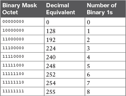
Table 4: Nine Possible Values in One Octet of a Subnet Mask
Many subnetting processes can be done with or without binary math. Some of those processes—mask conversion included—use the information in Table 4. You should plan to memorize the information in the table. I recommend making a copy of the table to keep handy while you practice. (You will likely memorize the contents of this table simply by practicing the conversion process enough to get both good and fast at the conversion.)
Using the table, the conversion processes in each direction with binary and decimal masks are as follows:
Binary to decimal: Organize the bits into four sets of eight. For each octet, find the binary value in the table and write down the corresponding decimal value.
Decimal to binary: For each octet, find the decimal value in the table and write down the corresponding 8-bit binary value.
Tables 5 and 6 show some examples

Table 5: Conversion Example: Binary to Decimal

Table 6: Conversion Examples: Decimal to Binar
Converting Between Prefix and DDN Masks
When learning, the best way to convert between the prefix and decimal formats is to first convert to binary. For example, to move from decimal to prefix, first convert decimal to binary and then from binary to prefix.
For the exams, set a goal to master these conversions doing the math in your head. While learning, you will likely want to use paper. To train yourself to do all this without writing it down, instead of writing each octet of binary, just write the number of binary 1s in that octet.
Figure 1 shows an example with a prefix-to-decimal conversion. The left side shows the conversion to binary as an interim step. For comparison, the right side shows the binary interim step in shorthand that just lists the number of binary 1s in each octet of the binary mask.

Figure 1: Conversion from Prefix to Decimal: Full Binary Versus Shorthand
Similarly, when converting from decimal to prefix, mentally convert to binary along the way, and as you improve, just think of the binary as the number of 1s in each octet. Figure 2 shows an example of such a conversion.

Figure 2: Conversion from Decimal to Prefix: Full Binary Versus Shorthand
Practice Converting Subnet Masks
Before moving to the second half of this lesson, and thinking about what these subnet masks mean, first do some practice. Practice the processes discussed in this lesson until you get the right answer most of the time. Later, before taking the exam, practice more until you master the topics in this lesson and can move pretty fast, as outlined in the right column of Table 7.

Table 7: Keep-Reading and Take-Exam Goals for This Lesson’s Topics
Table 8 lists eight practice problems. The table has three columns, one for each mask format. Each row lists one mask, in one format. Your job is to find the mask’s value in the other two formats for each row.

Table 8: Practice Problems: Find the Mask Values in the Other Two Formats
Identifying Subnet Design Choices Using Masks
Subnet masks have many purposes. In fact, if ten experienced network engineers were independently asked, “What is the purpose of a subnet mask?” the engineers would likely give a variety of true answers. The subnet mask plays several roles.
This lesson focuses on one particular use of a subnet mask: defining the prefix part of the IP addresses in a subnet. The prefix part must be the same value for all addresses in a subnet. In fact, a single subnet can be defined as all IPv4 addresses that have the same value in the prefix part of their IPv4 addresses.
While the previous paragraph might sound a bit formal, the idea is relatively basic, as shown in Figure 3. The figure shows a network diagram, focusing on two subnets: a subnet of all addresses that begin with 172.16.2 and another subnet made of all addresses that begin with 172.16.3. In this example, the prefix—the part that has the same value in all the addresses in the subnet—is the first three octets.

Figure 3: Simple Subnet Design, with Mask /24
While people can sit around a conference table and talk about how a prefix is three octets long, computers communicate that same concept using a subnet mask. In this case, the subnets use a subnet mask of /24, which means that the prefix part of the addresses is 24 bits (3 octets) long.
This section explains more about how to use a subnet mask to understand this concept of a prefix part of an IPv4 address, along with these other uses for a subnet mask. Note that this section discusses the first five items in the list.
- Defines the size of the prefix (combined network and subnet) part of the addresses in a subnet
- Defines the size of the host part of the addresses in the subnet
- Can be used to calculate the number of hosts in the subnet
- Provides a means for the network designer to communicate the design details—the number of subnet and host bits—to the devices in the network
- Under certain assumptions, can be used to calculate the number of subnets in the entire classful network
- Can be used in binary calculations of both the subnet ID and the subnet broadcast address
Masks Divide the Subnet’s Addresses into Two Parts
The subnet mask subdivides the IP addresses in a subnet into two parts: the prefix, or subnet part, and the host part.
The prefix part identifies the addresses that reside in the same subnet, because all IP addresses in the same subnet have the same value in the prefix part of their addresses. The idea is much like the postal code (ZIP codes in the United States) in mailing addresses. All mailing addresses in the same town have the same postal code. Likewise, all IP addresses in the same subnet have identical values in the prefix part of their addresses.
The host part of an address identifies the host uniquely inside the subnet. If you compare any two IP addresses in the same subnet, their host parts will differ, even though the prefix parts of their addresses have the same value. To summarize these key comparisons:
- Prefix (subnet) part: Equal in all addresses in the same subnet.
- Host part: Different in all addresses in the same subnet.
For example, imagine a subnet that, in concept, includes all addresses whose first three octets are 10.1.1. So, the following list shows several addresses in this subnet:
- 10.1.1.1
- 10.1.1.2
- 10.1.1.3
In this list, the prefix or subnet part (the first three octets of 10.1.1) are equal. The host part (the last octet [in bold]) is different. So, the prefix or subnet part of the address identifies the group, and the host part identifies the specific member of the group.
The subnet mask defines the dividing line between the prefix and the host part. To do so, the mask creates a conceptual line between the binary 1s in the binary mask and the binary 0s in the mask. In short, if a mask has P binary 1s, the prefix part is P bits long and the rest of the bits are host bits. Figure 4 shows the general concept.

Figure 4: Prefix (Subnet) and Host Parts Defined by Masks 1s and 0s
The next figure, Figure 5, shows a specific example using mask 255.255.255.0. Mask 255.255.255.0 (/24) has 24 binary 1s, for a prefix length of 24 bits.

Figure 5: Mask 255.255.255.0: P=24, H=8
Masks and Class Divide Addresses into Three Parts
In addition to the two-part view of IPv4 addresses, you can also think about IPv4 addresses as having three parts. To do so, just apply Class A, B, and C rules to the address format to define the network part at the beginning of the address. This added logic divides the prefix into two parts: the network part and the subnet part. The class defines the length of the network part, with the subnet part simply being the rest of the prefix. Figure 6 shows the idea.

Figure 6: Class Concepts Applied to Create Three Parts
The combined network and subnet parts act like the prefix because all addresses in the same subnet must have identical values in the network and subnet parts. The size of the host part remains unchanged, whether viewing the addresses as having two parts or three parts.
To be complete, Figure 7 shows the same example as in the previous section, with the subnet of “all addresses that begin with 10.1.1.” In that example, the subnet uses mask 255.255.255.0, and the addresses are all in Class A network 10.0.0.0. The class defines 8 network bits, and the mask defines 24 prefix bits, meaning that 24 – 8 = 16 subnet bits exist. The host part remains as 8 bits per the mask.

Figure 7: Subnet 10.1.1.0, Mask 255.255.255.0: N=8, S=16, H=8
Classless and Classful Addressing
The terms classless addressing and classful addressing refer to the two different ways to think about IPv4 addresses as described so far in this lesson. Classful addressing means that you think about Class A, B, and C rules, so the prefix is separated into the network and subnet parts, as shown in Figures 6 and 7. Classless addressing means that you ignore the Class A, B, and C rules and treat the prefix part as one part, as shown in Figures 4 and 5. The following more formal definitions are listed for reference and study:
- Classless addressing: The concept that an IPv4 address has two parts—the prefix part plus the host part—as defined by the mask, with no consideration of the class (A, B, or C).
- Classful addressing: The concept that an IPv4 address has three parts—network, subnet, and host—as defined by the mask and Class A, B, and C rules
NOTE: Unfortunately, the networking world uses the terms classless and classful in a couple of different ways. In addition to the classless and classful addressing described here, each routing protocol can be categorized as either a classless routing protocol or a classful routing protocol. In addition, the terms classless routing and classful routing refer to some details of how Cisco routers forward (route) packets using the default route in some cases. As a result, these terms can be easily confused and misused. So, when you see the words classless and classful, be careful to note the context: addressing, routing, or routing protocols.
Calculations Based on the IPv4 Address Format
After you know how to break an address down using both classless and classful addressing rules, you can easily calculate a couple of important facts using some basic math formulas.
First, for any subnet, after you know the number of host bits, you can calculate the number of host IP addresses in the subnet. Next, if you know the number of subnet bits (using classful addressing concepts) and you know that only one subnet mask is used throughout the network, you can also calculate the number of subnets in the network. The formulas just require that you know the powers of 2:
Hosts in the subnet: 2H – 2, where H is the number of host bits.
Subnets in the network: 2s, where S is the number of subnet bits. Only use this formula if only one mask is used throughout the network.
The sizes of the parts of IPv4 addresses can also be calculated. The math is basic, but the concepts are important. Keeping in mind that IPv4 addresses are 32 bits long, the two parts with classless addressing must add up to 32 (P + H = 32), and with classful addressing, the three parts must add up to 32 (N + S + H = 32). Figure 8 shows the relationships.

Figure 8: Relationship Between /P, N, S, and H
You often begin with an IP address and mask, both when answering questions on the CCNA Routing and Switching exams and when examining problems that occur in real networks. Based on the information in this lesson and earlier lessons, you should be able to find all the information in Figure 8 and then calculate the number of hosts/subnet and the number of subnets in the network. For reference, the following process spells out the steps:
- Step 1. Convert the mask to prefix format (/P) as needed. (See the earlier section “Practice Converting Subnet Masks” for review.)
- Step 2. Determine N based on the class.
- Step 3. Calculate S = P – N.
- Step 4. Calculate H = 32 – P.
- Step 5. Calculate hosts/subnet: 2H – 2.
- Step 6. Calculate number of subnet: 2s.
For example, consider the case of IP address 8.1.4.5 with mask 255.255.0.0. Following the process:
- Step 1. 255.255.0.0 = /16, so P=16.
- Step 2. 8.1.4.5 is in the range 1–126 in the first octet, so it is Class A; so N=8.
- Step 3. S = P – N = 16 – 8 = 8.
- Step 4. H = 32 – P = 32 – 16 = 16.
- Step 5. 216 – 2 = 65,534 hosts/subnet.
- Step 6. 28 = 256 subnets.
Figure 9 shows a visual analysis of the same problem.

Figure 9 Visual Representation of Problem: 8.1.4.5, 255.255.0.0
For another example, consider address 200.1.1.1, mask 255.255.255.252. Following the process:
- Step 1. 255.255.255.252 = /30, so P=30.
- Step 2. 200.1.1.1 is in the range 192–223 in the first octet, so it is Class C; so N=24.
- Step 3. S = P – N = 30 – 24 = 6.
- Step 4. H = 32 – P = 32 – 30 = 2.
- Step 5. 22 – 2 = 2 hosts/subnet
- Step 6. 26 = 64 subnets.
This example uses a popular mask for serial links, because serial links only require two host addresses, and the mask supports only two host addresses.
Practice Analyzing Subnet Masks
As with the other subnetting math in this course, using a two-phase approach may help. Take time now to practice until you feel like you understand the process. Then, before the exam, make sure you master the math. Table 9 summarizes the key concepts and suggestions for this two-phase approach.

Table 9 Keep-Reading and Take-Exam Goals for This Lesson’s Topics
On a piece of scratch paper, answer the following questions. In each case:
- Determine the structure of the addresses in each subnet based on the class and mask, using classful IP addressing concepts. In other words, find the size of the network, subnet, and host parts of the addresses.
- Calculate the number of hosts in the subnet.
- Calculate the number of subnets in the network, assuming that the same mask is used throughout.
- 8.1.4.5, 255.255.254.0
- 130.4.102.1, 255.255.255.0
- 199.1.1.100, 255.255.255.0
- 130.4.102.1, 255.255.252.0
- 199.1.1.100, 255.255.255.224

Analyzing Classful IPv4 Networks
INTERNOLD NETWORKS CCNA LIVE WEBCLASS (INCLW)
Analyzing Classful IPv4 Networks
Contents
Analyzing Classful IPv4 Networks
When operating a network, you often start investigating a problem based on an IP address and mask. Based on the IP address alone, you should be able to determine several facts about the Class A, B, or C network in which the IP address resides. These facts can be useful when troubleshooting some networking problems.
This lesson lists the key facts about classful IP networks and explains how to discover these facts. Following that, this lesson lists some practice problems. Before moving to the next lesson, you should practice until you can consistently determine all these facts, quickly and confidently, based on an IP address.
Classful Network Concepts
Imagine that you have a job interview for your first IT job. As part of the interview, you’re given an IPv4 address and mask: 10.4.5.99, 255.255.255.0. What can you tell the interviewer about the classful network (in this case, the Class A network) in which the IP address resides?
This section, the first of two major sections in this lesson, reviews the concepts of classful IP networks (in other words, Class A, B, and C networks). In particular, this lesson examines how to begin with a single IP address and then determine the following facts:
- Class (A, B, or C)
- Default mask
- Number of network octets/bits
- Number of host octets/bits
- Number of host addresses in the network
- Network ID
- Network broadcast address
- First and last usable address in the network
IPv4 Network Classes and Related Facts
IP version 4 (IPv4) defines five address classes. Three of the classes, Classes A, B, and C, consist of unicast IP addresses. Unicast addresses identify a single host or interface so that the address uniquely identifies the device. Class D addresses serve as multicast addresses, so that one packet sent to a Class D multicast IPv4 address can actually be delivered to multiple hosts. Finally, Class E addresses were originally intended for experimentation, but were changed to simply be reserved for future use. The class can be identified based on the value of the first octet of the address, as shown in Table 1.

Table 1: IPv4 Address Classes Based on First Octet Values
After you identify the class as either A, B, or C, many other related facts can be derived just through memorization. Table 2 lists that information for reference and later study; each of these concepts is described in this lesson.

Table 2: Key Facts for Classes A, B, and C
At times, some people today look back and wonder, “Are there 128 class A networks, with two reserved networks, or are there truly only 126 class A networks?” Frankly, the difference is unimportant, and the wording is just two ways to state the same idea. The important fact to know is that Class A network 0.0.0.0 and network 127.0.0.0 are reserved. In fact, they have been reserved since the creation of Class A networks, as listed in RFC 791 (published in 1981).
Although it may be a bit of a tangent, what is more interesting today is that over time, other newer RFCs have also reserved small pieces of the Class A, B, and C address space. So, tables like Table 2, with the count of the numbers of Class A, B, and C networks, are a good place to get a sense of the size of the number; however, the number of reserved networks does change slightly over time (albeit slowly) based on these other reserved address ranges.
NOTE: If you are interested in seeing all the reserved IPv4 address ranges, just do an Internet search on “IANA IPv4 special-purpose address registry.”
The Number and Size of the Class A, B, and C Networks
Table 2 lists the range of Class A, B, and C network numbers; however, some key points can be lost just referencing a table of information. This section examines the Class A, B, and C network numbers, focusing on the more important points and the exceptions and unusual cases.
First, the number of networks from each class significantly differs. Only 126 Class A networks exist: network 1.0.0.0, 2.0.0.0, 3.0.0.0, and so on, up through network 126.0.0.0. However, 16,384 Class B networks exist, with more than 2 million Class C networks.
Next, note that the size of networks from each class also significantly differs. Each Class A network is relatively large—over 16 million host IP addresses per network—so they were originally intended to be used by the largest companies and organizations. Class B networks are smaller, with over 65,000 hosts per network. Finally, Class C networks, intended for small organizations, have 254 hosts in each network. Figure 1 summarizes those facts.

Figure 1: Numbers and Sizes of Class A, B, and C Networks
Address Formats
In some cases, an engineer might need to think about a Class A, B, or C network as if the network has not been subdivided through the subnetting process. In such a case, the addresses in the classful network have a structure with two parts: the network part (sometimes called the prefix) and the host part. Then, comparing any two IP addresses in one network, the following observations can be made:
- The addresses in the same network have the same values in the network part.
- The addresses in the same network have different values in the host part.
For example, in Class A network 10.0.0.0, by definition, the network part consists of the first octet. As a result, all addresses have an equal value in the network part, namely a 10 in the first octet. If you then compare any two addresses in the network, the addresses have a different value in the last three octets (the host octets). For example, IP addresses 10.1.1.1 and 10.1.1.2 have the same value (10) in the network part, but different values in the host part.
Figure 2 shows the format and sizes (in number of bits) of the network and host parts of IP addresses in Class A, B, and C networks, before any subnetting has been applied.

Figure 2: Sizes (Bits) of the Network and Host Parts of Unsubnetted Classful Networks
Default Masks
Although we humans can easily understand the concepts behind Figure 2, computers prefer numbers. To communicate those same ideas to computers, each network class has an associated default mask that defines the size of the network and host parts of an unsubnetted Class A, B, and C network. To do so, the mask lists binary 1s for the bits considered to be in the network part and binary 0s for the bits considered to be in the host part.
For example, Class A network 10.0.0.0 has a network part of the first single octet (8 bits) and a host part of last three octets (24 bits). As a result, the Class A default mask is 255.0.0.0, which in binary is
11111111 00000000 00000000 00000000
Figure 3 shows default masks for each network class, both in binary and dotted-decimal format.

Figure 3: Default Masks for Classes A, B, and C
NOTE: Decimal 255 converts to the binary value 11111111. Decimal 0, converted to 8-bit binary, is 00000000. See “Numeric Reference Tables,” for a conversion table.
Number of Hosts per Network
Calculating the number of hosts per network requires some basic binary math. First, consider a case where you have a single binary digit. How many unique values are there? There are, of course, two values: 0 and 1. With 2 bits, you can make four combinations: 00, 01, 10, and 11. As it turns out, the total combination of unique values you can make with N bits is 2N.
Host addresses—the IP addresses assigned to hosts—must be unique. The host bits exist for the purpose of giving each host a unique IP address by virtue of having a different value in the host part of the addresses. So, with H host bits, 2H unique combinations exist.
However, the number of hosts in a network is not 2H; instead, it is 2H – 2. Each network reserves two numbers that would have otherwise been useful as host addresses, but have instead been reserved for special use: one for the network ID and one for the network broadcast address. As a result, the formula to calculate the number of host addresses per Class A, B, or C network is
2H – 2
where H is the number of host bits.
Deriving the Network ID and Related Numbers
Each classful network has four key numbers that describe the network. You can derive these four numbers if you start with just one IP address in the network. The numbers are as follows:
- Network number
- First (numerically lowest) usable address
- Last (numerically highest) usable address
- Network broadcast address
First, consider both the network number and first usable IP address. The network number, also called the network ID or network address, identifies the network. By definition, the network number is the numerically lowest number in the network. However, to prevent any ambiguity, the people that made up IP addressing added the restriction that the network number cannot be assigned as an IP address. So, the lowest number in the network is the network ID. Then, the first (numerically lowest) host IP address is one larger than the network number.
Next, consider the network broadcast address along with the last (numerically highest) usable IP address. The TCP/IP RFCs define a network broadcast address as a special address in each network. This broadcast address could be used as the destination address in a packet, and the routers would forward a copy of that one packet to all hosts in that classful network. Numerically, a network broadcast address is always the highest (last) number in the network. As a result, the highest (last) number usable as an IP address is the address that is simply one less than the network broadcast address.
Simply put, if you can find the network number and network broadcast address, finding the first and last usable IP addresses in the network is easy. For the exam, you should be able to find all four values with ease; the process is as follows:
Step 1. Determine the class (A, B, or C) based on the first octet.
Step 2. Mentally divide the network and host octets based on the class.
Step 3. To find the network number, change the IP address’s host octets to 0.
Step 4. To find the first address, add 1 to the fourth octet of the network ID.
Step 5. To find the broadcast address, change the network ID’s host octets to 255.
Step 6. To find the last address, subtract 1 from the fourth octet of the network broadcast address.
The written process actually looks harder than it is. Figure 4 shows an example of the process, using Class A IP address 10.17.18.21, with the circled numbers matching the process.

Figure 4: Example of Deriving the Network ID and Other Values from 10.17.18.21
Figure 4 shows the identification of the class as Class A (Step 1) and the number of network/host octets as 1 and 3, respectively. So, to find the network ID at Step 3, the figure copies only the first octet, setting the last three (host) octets to 0. At Step 4, just copy the network ID and add 1 to the fourth octet. Similarly, to find the broadcast address at Step 5, copy the network octets, but set the host octets to 255. Then, at Step 6, subtract 1 from the fourth octet to find the last (numerically highest) usable IP address.
Just to show an alternative example, consider IP address 172.16.8.9. Figure 5 shows the process applied to this IP address.

Figure 5: Example Deriving the Network ID and Other Values from 172.16.8.9
Figure 5 shows the identification of the class as Class B (Step 1) and the number of network/host octets as 2 and 2, respectively. So, to find the network ID at Step 3, the figure copies only the first two octets, setting the last two (host) octets to 0. Similarly, Step 5 shows the same action, but with the last two (host) octets being set to 255.
Unusual Network IDs and Network Broadcast Addresses
Some of the more unusual numbers in and around the range of Class A, B, and C network numbers can cause some confusion. This section lists some examples of numbers that make many people make the wrong assumptions about the meaning of the number.
For Class A, the first odd fact is that the range of values in the first octet omits the numbers 0 and 127. As it turns out, what would be Class A network 0.0.0.0 was originally reserved for some broadcasting requirements, so all addresses that begin with 0 in the first octet are reserved. What would be Class A network 127.0.0.0 is still reserved because of a special address used in software testing, called the loopback address (127.0.0.1).
For Class B (and C), some of the network numbers can look odd, particularly if you fall into a habit of thinking that 0s at the end means the number is a network ID, and 255s at the end means it’s a network broadcast address. First, Class B network numbers range from 128.0.0.0 to 191.255.0.0, for a total of 214 networks. However, even the very first (lowest number) Class B network number (128.0.0.0) looks a little like a Class A network number, because it ends with three 0s. However, the first octet is 128, making it a Class B network with a two-octet network part (128.0).
For another Class B example, the high end of the Class B range also might look strange at first glance (191.255.0.0), but this is indeed the numerically highest of the valid Class B network numbers. This network’s broadcast address, 191.255.255.255, might look a little like a Class A broadcast address because of the three 255s at the end, but it is indeed the broadcast address of a Class B network.
Similarly to Class B networks, some of the valid Class C network numbers do look strange. For example, Class C network 192.0.0.0 looks a little like a Class A network because of the last three octets being 0, but because it is a Class C network, it consists of all addresses that begin with three octets equal to 192.0.0. Similarly, Class C network 223.255.255.0, another valid Class C network, consists of all addresses that begin with 223.255.255.
Practice with Classful Networks
As with all areas of IP addressing and subnetting, you need to practice to be ready for the CCENT and CCNA Routing and Switching exams. You should practice some while reading this lesson to make sure that you understand the processes. At that point, you can use your notes and this course as a reference, with a goal of understanding the process. After that, keep practicing this and all the other subnetting processes. Before you take the exam, you should be able to always get the right answer, and with speed. Table 3 summarizes the key concepts and suggestions for this two-phase approach.

Table 3: Keep-Reading and Take-Exam Goals for This Lesson’s Topics
Practice Deriving Key Facts Based on an IP Address
Practice finding the various facts that can be derived from an IP address, as discussed throughout this lesson. To do so, complete Table 4.

Table 4: Practice Problems: Find the Network ID and Network Broadcast
The answers are listed in the section “Answers to Earlier Practice Problems,” later in this lesson.
Practice Remembering the Details of Address Classes
Tables 1 and 2, shown earlier in this lesson, summarized some key information about IPv4 address classes. Tables 5 and 6 show sparse versions of these same tables. To practice recalling those key facts, particularly the range of values in the first octet that identifies the address class, complete these tables. Then, refer to Tables 1 and 2 to check your answers. Repeat this process until you can recall all the information in the tables.

Table 5: Sparse Study Table Version of Table 1

Table 6: Sparse Study Table Version of Table 2

INCLW01 Week 2 Practice Quiz
INTERNOLD NETWORKS CCNA LIVE WEBCLASS (INCLW)
week 2 practice quiz

Read the question carefully and choose the best answer(s).
Note: This is a mini-quiz of 10 questions per attempt. Always click 'Try Again' to get a new sets of questions.
Miscellaneous LAN Topics
INTERNOLD NETWORKS CCNA LIVE WEBCLASS (INCLW)
Miscellaneous LAN Topics
Contents
Miscellaneous LAN Topics
Between this book and the ICND1 100-105 Cert Guide, 14 chapters have been devoted to topics specific to LANs. This chapter is the last of those chapters. This chapter completes the LAN-specific discussion with a few small topics that just do not fit neatly in the other chapters.
The chapter begins with three security topics. The first section addresses IEEE 802.1x, which defines a mechanism to secure user access to a LAN by requiring the user to supply a username and password before a switch allows the device’s sent frames into the LAN. This tool helps secure the network against attackers gaining access to the network. The second section, “AAA Authentication,” discusses network device security, protecting router and switch CLI access by requiring username/password login with an external authentication server. The third section, “DHCP Snooping,” explores how switches can prevent security attacks that take advantage of DHCP messages and functions. By watching DHCP messages, noticing when they are used in abnormal ways not normally done with DHCP, DHCP can prevent attacks by simply filtering certain DHCP messages.
The final of the four major sections in this chapter looks at two similar design tools that make multiple switches act like one switch: switch stacking and chassis aggregation. Switch stacking allows a set of similar switches that sit near to each other (in the same wiring closet, typically in the same part of the same rack) to be cabled together and then act like a single switch. Using a switch stack greatly reduces the amount of work to manage the switch, and it reduces the overhead of control and management protocols used in the network. Switch chassis aggregation has many of the same benefits, but is supported more often as a distribution or core switch feature, with switch stacking as a more typical access layer switch feature.
All four sections of this chapter have a matching exam topic that uses the verb “describe,” so this chapter touches on the basic descriptions of a tool, rather than deep configuration. A few of the topics will show some configuration as a means to describe the topic, but the chapter is meant to help you come away with an understanding of the fundamentals, rather than an ability to configure the features.
Securing Access with IEEE 802.1x
In some enterprise LANs, the LAN is built with cables run to each desk, in every cubicle and every office. When you move to a new space, all you have to do is connect a short patch cable from your PC to the RJ-45 socket on the wall and you are connected to the network. Once booted, your PC can send packets anywhere in the network. Security? That happens mostly at the devices you try to access, for instance, when you log in to a server.
That previous paragraph is true of how many networks work. That attitude views the network as an open highway between the endpoints in the network, and the network is there to create connectivity, with high availability, and to make it easy to connect your device. Those goals are worthy goals. However, making the LAN accessible to anyone, so that anyone can attempt to connect to servers in the network, allows attackers to connect and then try and break in to the security that protects the server. That approach may be too insecure. For instance, any attacker who could gain physical access could plug in his laptop and start running tools to try to exploit all those servers attached to the internal network.
Today, many companies secure access to the network. Sure, they begin by creating basic connectivity: cabling the LAN and connecting cables to all the desks at all the cubicles and offices. All those ports physically work. But a user cannot just plug in her PC and start working; she must go through a security process before the LAN switch will allow the user to send any other messages in the network.
Switches can use IEEE standard 802.1x to secure access to LAN ports. To set up the feature, the LAN switches must be configured to enable 802.1x. Additionally, the IT staff must implement an authentication, authorization, and accounting (AAA) server. The AAA server (commonly pronounced “triple A” server) will keep the usernames and passwords, and when the user supplies that information, it is the AAA server that determines if what the user typed was correct or not.
Once implemented, the LAN switch acts as an 802.1x authenticator, as shown in Figure 6-1. As an 802.1x authenticator, a switch can be configured to enable some ports for 802.1x, most likely the access ports connected to end users. Enabling a port for 802.1x defines that when the port first comes up, the switch filters all incoming traffic (other than 802.1x traffic). 802.1x must first authenticate the user that uses that device.

Switch as 802.1x Authenticator, with AAA Server, and PC Not Yet Connected
Note that the switch usually configures access ports that connect to end users with 802.1x, but does not enable 802.1x on ports connected to IT-controlled devices, such as trunk ports, or ports connected in parts of the network that are physically more secure.
The 802.1x authentication process works like the flow in Figure 6-2. Once the PC connects and the port comes up, the switch uses 802.1x messages to ask the PC to supply a username/password. The PC user must then supply that information. For that process to work, the end-user device must be using an 802.1x client called a supplicant; many OSs include an 802.1x supplicant, so it may just be seen as a part of the OS settings.

Generic 802.1x Authentication Flows
At Steps 3 and 4 in Figure 6-2, the switch authenticates the user, to find out if the username and password combination is legitimate. The switch, acting as 802.1x authenticator, asks the AAA server if the supplied username and password combo is correct, with the AAA server answering back. If the username and password were correct, then the switch authorizes the port. Once authorized, the switch no longer filters incoming messages on that port. If the username/password check shows that the username/password was incorrect, or the process fails for any reason, the port remains in an unauthorized state. The user can continue to retry the attempt.
Figure 6-3 rounds out this topic by showing an example of one key protocol used by 802.1x: Extensible Authentication Protocol (EAP). The switch (the authenticator) uses RADIUS between itself and the AAA server, which itself uses IP and UDP. However, 802.1x, an Ethernet protocol, does not use IP or UDP. But 802.1x wants to exchange some authentication information all the way to the RADIUS AAA server. The solution is to use EAP, as shown in Figure 6-3.

EAP and Radius Protocol Flows with 802.1x
As shown in the figure, the EAP message flows from the supplicant to the authentication server, just in different types of messages. The flow from the supplicant (the end-user device) to the switch transports the EAP message directly in an Ethernet frame with an encapsulation called EAP over LAN (EAPoL). The flow from the authenticator (switch) to the authentication server flows in an IP packet. In fact, it looks much like a normal message used by the RADIUS protocol (RFC 2865). The RADIUS protocol works as a UDP application, with an IP and UDP header, as shown in the figure.
Now that you have heard some of the details and terminology, this list summarizes the entire process:
A AAA server must be configured with usernames and passwords.
Each LAN switch must be enabled for 802.1x, to enable the switch as an authenticator, to configure the IP address of the AAA server, and to enable 802.1x on the required ports.
Users must know a username/password combination that exists on the AAA server, or they will not be able to access the network from any device.
AAA Authentication
The ICND1 100-105 Cert Guide discusses many details about device management, in particular how to secure network devices. However, all those device security methods shown in the ICND1 half of the CCNA R&S exam topics use locally configured information to secure the login to the networking device.
Using locally configured usernames and passwords configured on the switch causes some administrative headaches. For instance, every switch and router needs the configuration for all users who might need to log in to the devices. Good security practices tell us to change our passwords regularly, but logging in to hundreds of devices to change passwords is a large task, so often, the passwords remain unchanged for long periods.
A better option would be to use an external AAA server. The AAA server centralizes and secures all the username/password pairs. The switches and routers still need some local security configuration to refer to the AAA server, but the username/password exist centrally, greatly reducing the administrative effort, and increasing the chance that passwords are changed regularly and are more secure. It is also easier to track which users logged in to which devices and when, and to revoke access as people leave their current job.
This short section discusses the basics of how networking devices can use a AAA server.
AAA Login Process
First, to use AAA, the site would need to install and configure a AAA server, such as the Cisco Access Control Server (ACS). Cisco ACS is AAA software that you can install on your own server (physical or virtual).
The networking devices would each then need new configuration to tell the device to start using the AAA server. That configuration would point to the IP address of the AAA server, and define which AAA protocol to use: either TACACS+ or RADIUS. The configuration includes details about TCP (TACACS+) or UDP (RADIUS) ports to use.
When using a AAA server for authentication, the switch (or router) simply sends a message to the AAA server asking whether the username and password are allowed, and the AAA server replies. Figure 6-4 shows an example, with the user first supplying his username/password, the switch asking the AAA server, and the server replying to the switch stating that the username/password is valid.

Basic Authentication Process with an External AAA Server
TACACS+ and RADIUS Protocols
While Figure 6-4 shows the general idea, note that the information flows with a couple of different protocols. On the left, the connection between the user and the switch or router uses Telnet or SSH. On the right, the switch and AAA server typically use either the RADIUS or TACACS+ protocol, both of which encrypt the passwords as they traverse the network.
The AAA server can also provide authorization and accounting features as well. For instance, for networking devices, IOS can be configured so that each user can be allowed to use only a specific subset of CLI commands. So, instead of having basically two levels of authority—user mode and privileged mode—each device can configure a custom set of command authority settings per user. Alternately, those details can be centrally configured at the AAA server, rather than configuring the details at each device. As a result, different users can be allowed to use different subsets of the commands, but as identified through requests to the AAA server, rather than repetitive laborious configuration on every device. (Note that TACACS+ supports this particular command authorization function, whereas RADIUS does not.)
Table 6-2 lists some basic comparison points between TACACS+ and RADIUS.

Comparisons Between TACACS+ and RADIUS
AAA Configuration Examples
Learning how to configure a router or switch to use a AAA server can be difficult. AAA requires that you learn several new commands. Besides all that, enabling AAA actually changes the rules used on a router for login authentication—for instance, you cannot just add a login command on the console line anymore after you have enabled AAA.
The exam topics use the phrase “describe” regarding AAA features, rather than configure, verify, or troubleshoot. However, to understand AAA on switches or routers, it helps to work through an example configuration. This next topic focuses on the big ideas behind a AAA configuration, instead of worrying about working through all the parameters, verifying the results, or memorizing a checklist of commands. The goal is to help you see how AAA on a switch or router changes login security.
NOTE: Throughout this book and the ICND1 Cert Guide, the login security details work the same on both routers and switches, with the exception that switches do not have an auxiliary port, whereas routers often do. But the configuration works the same on both routers and switches, so when this section mentions a switch for login security, the same concept applies to routers as well.
Everything you learned about switch login security for ICND1 in the ICND1 Cert Guide assumed an unstated default global command: no aaa new-model. That is, you had not yet added the aaa new-model global command to the configuration. Configuring AAA requires the aaa new-model command, and this single global command changes how that switch does login security.
The aaa new-model global command enables AAA services in the local switch (or router). It even enables new commands, commands that would not have been accepted before, and that would not have shown up when getting help with a question mark from the CLI. The aaa new-model command also changes some default login authentication settings. So, think of this command as the dividing line between using the original simple ways of login security versus a more advanced method.
After configuring the aaa new-model command on a switch, you need to define each AAA server, plus configure one or more groups of AAA servers aptly named a AAA group. For each AAA server, configure its IP address and a key, and optionally the TCP or UDP port number used, as seen in the middle part of Figure 6-5. Then you create a server group for each group of AAA servers to group one or more AAA servers, as seen in the bottom of Figure 6-5. (Other configuration settings will then refer to the AAA server group rather than the AAA server.)

Enabling AAA and Defining AAA Servers and Groups
The configuration concepts in Figure 6-5 still have not completed the task of configuring AAA authentication. IOS uses the following additional logic to connect the rest of the logic:
IOS does login authentication for the console, vty, and aux port, by default, based on the setting of the aaa authentication login default global command.
The aaa authentication login default method1 method2... global command lists different authentication methods, including referencing a AAA group to be used (as shown at the bottom of Figure 6-5).
The methods include: a defined AAA group of AAA servers; local, meaning a locally configured list of usernames/passwords; or line, meaning to use the password defined by the password line subcommand.
Basically, when you want to use AAA for login authentication on the console or vty lines, the most straightforward option uses the aaa authentication login default command. As Figure 6-6 shows with this command, it lists multiple authentication methods. The switch tries the first method, and if that method returns a definitive answer, the process is done. However, if that method is not available (for instance, none of the AAA servers is reachable over the IP network), IOS on the local device moves on to the next method.

Default Login Authentication Rules
The idea of defining at least a couple of methods for login authentication makes good sense. For instance, the first method could be a AAA group so that each engineer logs in to each device with that engineer’s unique username and password. However, you would not want the engineer to fail to log in just because the IP network is having problems and the AAA servers cannot send packets back to the switch. So, using a backup login method (a second method listed in the command) makes good sense.
Figure 6-7 shows three sample commands for perspective. All three commands reference the same AAA group (WO-AAA-Group). The command labeled with a 1 in the figure takes a shortsighted approach, using only one authentication method with the AAA group. Command 2 in the figure uses two authentication methods: one with AAA and a second method (local). (This command’s local keyword refers to the list of local username commands as configured on the local switch.) Command 3 in the figure again uses a AAA group as the first method, followed by the keyword login, which tells IOS to use the password line subcommand.

Examples of AAA Login Authentication Method Combinations
DHCP Snooping
To understand the kinds of risks that exist in modern networks, you have to first understand the rules. Then you have to think about how an attacker might take advantage of those rules in different ways. Some attacks might cause harm, and might be called a denial-of-service (DoS) attack. Or an attacker may gather more data to prepare for some other attack. Whatever the goal, for every protocol and function you learn in networking, there are possible methods to take advantage of those features to give an attacker an advantage.
Cisco chose to add one exam topic for this current CCNA R&S exam that focuses on mitigating attacks based on a specific protocol: DHCP. DHCP has become a very popular protocol, used in most every enterprise, home, and service provider. As a result, attackers have looked for methods to take advantage of DHCP. One way to help mitigate the risks of DHCP is to use a LAN switch feature called DHCP snooping.
This third of four major sections of the chapter works through the basics of DHCP snooping. It starts with the main idea, and then shows one example of how an attacker can misuse DHCP to gain an advantage. The last section explains the logic used by DHCP snooping.
DHCP Snooping Basics
DHCP snooping on a switch acts like a firewall or an ACL in many ways. It will watch for incoming messages on either all ports or some ports (depending on the configuration). It will look for DHCP messages, ignoring all non-DHCP messages and allowing those through. For any DHCP messages, the switch’s DHCP snooping logic will make a choice: allow the message or discard the message.
To be clear, DHCP snooping is a Layer 2 switch feature, not a router feature. Specifically, any switch that performs Layer 2 switching, whether it does only Layer 2 switching or acts as a multilayer switch, typically supports DHCP snooping. DHCP snooping must be done on a device that sits between devices in the same VLAN, which is the role of a Layer 2 switch rather than a Layer 3 switch or router.
The first big idea with DHCP snooping is the idea of trusted ports and untrusted ports. To understand why, ponder for a moment all the devices that might be connected to one switch. The list includes routers, servers, and even other switches. It includes end-user devices, such as PCs. It includes wireless access points, which in turn connect to end-user devices. Figure 6-8 shows a representation.

DHCP Snooping Basics: Client Ports Are Untrusted
DHCP snooping begins with the assumption that end-user devices are untrusted, while devices more within the control of the IT department are trusted. However, a device on an untrusted port can still use DHCP. Instead, making a port untrusted for DHCP snooping means this:
Watch for incoming DHCP messages, and discard any that are considered to be abnormal for an untrusted port and therefore likely to be part of some kind of attack.
An Example DHCP-based Attack
To give you perspective, Figure 6-9 shows a legitimate user’s PC on the far right and the legitimate DHCP sever on the far left. However, an attacker has connected his laptop to the LAN and started his DHCP attack. Remember, PC1’s first DHCP message will be a LAN broadcast, so the attacker’s PC will receive those LAN broadcasts from any DHCP clients like PC1. (In this case, assume PC1 is attempting to lease an IP address while the attacker is making his attack.)

DHCP Attack Supplies Good IP Address but Wrong Default Gateway
In this example, the DHCP server created and used by the attacker actually leases a useful IP address to PC1, in the correct subnet, with the correct mask. Why? The attacker wants PC1 to function, but with one twist. Notice the default gateway assigned to PC1: 10.1.1.2, which is the attacker’s PC address, rather than 10.1.1.1, which is R1’s address. Now PC1 thinks it has all it needs to connect to the network, and it does—but now all the packets sent by PC1 flow first through the attacker’s PC, creating a man-in-the-middle attack, as shown in Figure 6-10.

Unfortunate Result: DHCP Attack Leads to Man-in-the-Middle
The two steps in the figure show data flow once DHCP has completed. For any traffic destined to leave the subnet, PC1 sends its packets to its default gateway, 10.1.1.2, which happens to be the attacker. The attacker forwards the packets to R1. The PC1 user can connect to any and all applications just like normal, but now the attacker can keep a copy of anything sent by PC1.
How DHCP Snooping Works
The preceding example shows just one attack. Some attacks use an extra DHCP server (called a spurious DHCP server), and some attacks happen by using DHCP client functions in different ways. DHCP snooping considers how DHCP should work and filters out any messages that would not be part of a normal use of DHCP.
DHCP snooping needs a few configuration settings. First, the engineer enables DHCP snooping either globally on a switch or by VLAN (that is, enabled on some VLANs, and not on others). Once enabled, all ports are considered untrusted until configured as trusted.
Next, some switch ports need to be configured as trusted. Any switch ports connected to legitimate DHCP servers should be trusted. Additionally, ports connected to other switches, and ports connected to routers, should also be trusted. Why? Trusted ports are basically ports that could receive messages from legitimate DHCP servers in the network. The legitimate DHCP servers in a network are well known.
Just for a quick review, the ICND1 Cert Guide described the DHCP messages used in normal DHCP lease flows (DISCOVER, OFFER, REQUEST, ACK [DORA]). For these and other DHCP messages, a message is normally sent by either a DHCP client or a server, but not both. In the DORA messages, the client sends the DISCOVER and REQUEST, and the server sends the OFFER and ACK. Knowing that only DHCP servers should send DHCP OFFER and ACK messages, DHCP snooping allows incoming OFFER and ACK messages on trusted ports, but filters those messages if they arrive on untrusted ports.
So, the first rule of DHCP snooping is for the switch to trust any ports on which legitimate messages from trusted DHCP servers might arrive. Conversely, by leaving a port untrusted, the switch is choosing to discard any incoming DHCP server-only messages. Figure 6-11 summarizes these points, with the legitimate DHCP server on the left, on a port marked as trusted.

Summary of Rules for DHCP Snooping
The logic for untrusted DHCP ports is a little more challenging. Basically, the untrusted ports are the real user population, all of which rely heavily on DHCP. Those ports also include those few people trying to attack the network with DHCP, and you cannot predict which of the untrusted ports have legitimate users and which are attacking the network. So the DHCP snooping function has to watch the DHCP messages over time, and even keep some state information in a DHCP Binding Table, so that it can decide when a DHCP message should be discarded.
The DHCP Binding Table is a list of key pieces of information about each successful lease of an IPv4 address. Each new DHCP message received on an untrusted port can then be compared to the DHCP Binding Table, and if the switch detects conflicts when comparing the DHCP message to the Binding Table, then the switch will discard the message.
To understand more specifically, first look at Figure 6-12, which shows a switch building one entry in its DHCP Binding Table. In this simple network, the DHCP client on the right leases IP address 10.1.1.11 from the DHCP server on the left. The switch’s DHCP snooping feature combines the information from the DHCP messages, with information about the port (interface F0/2, assigned to VLAN 11 by the switch), and puts that in the DHCP Binding Table.

Legitimate DHCP Client with DHCP Binding Entry Built by DHCP Snooping
Because of this DHCP binding table entry, DHCP snooping would now prevent another client on another switch port from claiming to be using that same IP address (10.1.1.11) or the same MAC address (2000.1111.1111). (Many DHCP client attacks will use the same IP address or MAC address as a legitimate host.)
Note that beyond firewall-like rules of filtering based on logic, DHCP snooping can also be configured to rate limit the number of DHCP messages on an interface. For instance, by rate limiting incoming DHCP messages on untrusted interfaces, DHCP snooping can help prevent a DoS attack designed to overload the legitimate DHCP server, or to consume all the available DHCP IP address space.
Summarizing DHCP Snooping Features
DHCP snooping can help reduce risk, particularly because DHCP is such a vital part of most networks. The following list summarizes some of the key points about DHCP snooping for easier exam study:
Trusted ports: Trusted ports allow all incoming DHCP messages.
Untrusted ports, server messages: Untrusted ports discard all incoming messages that are considered server messages.
Untrusted ports, client messages: Untrusted ports apply more complex logic for messages considered client messages. They check whether each incoming DHCP message conflicts with existing DHCP binding table information and, if so, discard the DHCP message. If the message has no conflicts, the switch allows the message through, which typically results in the addition of new DHCP Binding Table entries.
Rate limiting: Optionally limits the number of received DHCP messages per second, per port.
Switch Stacking and Chassis Aggregation
Cisco offers several options that allow customers to configure their Cisco switches to act cooperatively to appear as one switch, rather than as multiple switches. This final major section of the chapter discusses two major branches of these technologies: switch stacking, which is more typical of access layer switches, and chassis aggregation, more commonly found on distribution and core switches.
Traditional Access Switching Without Stacking
Imagine for a moment that you are in charge of ordering all the gear for a new campus, with several multistory office buildings. You take a tour of the space, look at drawings of the space, and start thinking about where all the people and computers will be. At some point, you get to the point of thinking about how many Ethernet ports you need in each wiring closet.
Imagine for one wiring closet you need 150 ports today, and you want to build enough switch port capacity to 200 ports. What size switches do you buy? Do you get one switch for the wiring closet, with at least 200 ports in the switch? (The books do not discuss various switch models very much, but yes, you can buy LAN switches with hundreds of ports in one switch.) Or do you buy a pair of switches with at least 100 ports each? Or eight or nine switches with 24 access ports each?
There are pros and cons for using smaller numbers of large switches, and vice versa. To meet those needs, vendors such as Cisco offer switches with a wide range of port densities. However, a switch feature called switch stacking gives you some of the benefits of both worlds.
To appreciate the benefits of switch stacking, imagine a typical LAN design like the one shown in Figure 6-13. The figure shows the conceptual design, with two distribution switches and four access layer switches.

Typical Campus Design: Access Switches and Two Distribution Switches
For later comparison, let me emphasize a few points here. Access switches A1 through A4 all operate as separate devices. The network engineer must configure each. They each have an IP address for management. They each run CDP, STP, and maybe VTP. They each have a MAC address table, and they each forward Ethernet frames based on that MAC address table. Each switch probably has very similar configuration, but that configuration is separate, and all the functions are separate.
Now picture those same four access layer switches physically, not in Figure 6-13, but as you would imagine them in a wiring closet, even in the same rack. In this case, imagine all four access switches sit in the same rack in the same closet. All the wiring on that floor of the building runs back to the wiring closet, and each cable is patched into some port in one of these four switches. Each switch might be one rack unit (RU) tall (1.75 inches), and they all sit one on top of the other.
Switch Stacking of Access Layer Switches
The scenario described so far is literally a stack of switches one above the other. Switch stacking technology allows the network engineer to make that stack of physical switches act like one switch. For instance, if a switch stack was made from the four switches in Figure 6-13, the following would apply:
The stack would have a single management IP address.
The engineer would connect with Telnet or SSH to one switch (with that one management IP address), not multiple switches.
One configuration file would include all interfaces in all four physical switches.
STP, CDP, VTP would run on one switch, not multiple switches.
The switch ports would appear as if all are on the same switch.
There would be one MAC address table, and it would reference all ports on all physical switches.
The list could keep going much longer for all possible switch features, but the point is that switch stacking makes the switches act as if they are simply parts of a single larger switch.
To make that happen, the switches must be connected together with a special network. The network does not use standard Ethernet ports. Instead, the switches have special hardware ports called stacking ports. With the Cisco FlexStack and FlexStack-Plus stacking technology, a stacking module must be inserted into each switch, and then connected with a stacking cable.
NOTE: Cisco has created a few switch stacking technologies over the years, so to avoid having to refer to them all, note that this section describes Cisco’s FlexStack and FlexStack Plus options. These stacking technologies are supported to different degrees in the popular 2960-S, 2960-X, and 2960-XR switch families.
The stacking cables together make a ring between the switches as shown in Figure 6-14. That is, the switches connect in series, with the last switch connecting again to the first. Using full duplex on each link, the stacking modules and cables create two paths to forward data between the physical switches in the stack. The switches use these connections to communicate between the switches to forward frames and to perform other overhead functions.

Stacking Cables Between Access Switches in the Same Rack
Note that each stacking module has two ports with which to connect to another switch’s stacking module. For instance, if the four switches were all 2960XR switches, each would need one stacking module, and four cables total to connect the four switches as shown. Figure 6-15 shows the same idea in Figure 6-14, but as a photo that shows the stacking cables on the left side of the figure.

Photo of Four 2960X Switches Cabled on the Left with Stacking Cables
You should think of switch stacks as literally a stack of switches in the same rack. The stacking cables are short, with the expectation that the switches sit together in the same room and rack. For instance, Cisco offers stacking cables of .5, 1, and 3 meters long for the FlexStack and FlexStack-Plus stacking technology discussed in more depth at the end of this section.
Switch Stack Operation as a Single Logical Switch
With a switch stack, the switches together act as one logical switch. This term (logical switch) is meant to emphasize that there are obviously physical switches, but they act together as one switch.
To make it all work, one switch acts as a stack master to control the rest of the switches. The links created by the stacking cables allow the physical switches to communicate, but the stack master is in control of the work. For instance, if you number the physical switches as 1, 2, 3, and 4, a frame might arrive on switch 4 and need to exit a link on switch 3. If switch 1 were the stack master, switches 1, 3, and 4 would all need to communicate over the stack links to forward that frame. But switch 1, as stack master, would do the matching of the MAC address table to choose where to forward the frame.
Figure 6-16 focuses on the LAN design impact of how a switch stack acts like one logical switch. The figure shows the design with no changes to the cabling between the four access switches and the distribution switches. Formerly, each separate access switch had two links to the distribution layer: one connected to each distribution switch (see Figure 6-13). That cabling is unchanged. However, acting as one logical switch, the switch stack now operates as if it is one switch, with four uplinks to each distribution switch. Add a little configuration to put each set of four links into an EtherChannel, and you have the design shown in Figure 6-16.

Stack Acts Like One Switch
The stack also simplifies operations. Imagine for instance the scope of an STP topology for a VLAN that has access ports in all four of the physical access switches in this example. That Spanning Tree would include all six switches. With the switch stack acting as one logical switch, that same VLAN now has only three switches in the STP topology, and is much easier to understand and predict.
Cisco FlexStack and FlexStack-Plus
Just to put a finishing touch on the idea of a switch stack, this closing topic examines a few particulars of Cisco’s FlexStack and FlexStack-Plus stacking options.
Cisco’s stacking technologies require that Cisco plan to include stacking as a feature in a product, given that it requires specific hardware. Cisco has a long history of building new model series of switches with model numbers that begin with 2960. Per Cisco’s documentation, Cisco created one stacking technology, called FlexStack, as part of the introduction of the 2960-S model series. Cisco later enhanced FlexStack with FlexStack-Plus, adding support with products in the 2960-X and 2960-XR model series. For switch stacking to support future designs, the stacking hardware tends to increase over time as well, as seen in the comparisons between FlexStack and FlexStack-Plus in Table 6-3.

Comparisons of Cisco’s FlexStack and FlexStack-Plus Options
Chassis Aggregation
The term chassis aggregation refers to another Cisco technology used to make multiple switches operate as a single switch. From a big picture perspective, switch stacking is more often used and offered by Cisco in switches meant for the access layer. Chassis aggregation is meant for more powerful switches that sit in the distribution and core layers. Summarizing some of the key differences, chassis aggregation
Typically is used for higher-end switches used as distribution or core switches
Does not require special hardware adapters, instead using Ethernet interfaces
Aggregates two switches
Arguably is more complex but also more functional
The big idea of chassis aggregation is the same as for a switch stack: make multiple switches act like one switch, which gives you some availability and design advantages. But much of the driving force behind chassis aggregation is about high-availability design for LANs. This section works through a few of those thoughts to give you the big ideas about the thinking behind high availability for the core and distribution layer.
NOTE: This section looks at the general ideas of chassis aggregation, but for further reading about a specific implementation, search at Cisco.com for Cisco’s Virtual Switching System (VSS) that is supported on 6500 and 6800 series switches.
High Availability with a Distribution/Core Switch
Even without chassis aggregation, the distribution and core switches need to have high availability. The next few pages look at how the switches built for use as distribution and core switches can help improve availability, even without chassis aggregation.
If you were to look around a medium to large enterprise campus LAN, you would typically find many more access switches than distribution and core switches. For instance, you might have four access switches per floor, with ten floors in a building, for 40 access switches. That same building probably has only a pair of distribution switches.
And why two distribution switches instead of one? Because if the design used only one distribution switch, and it failed, none of the devices in the building could reach the rest of the network. So, if two distribution switches are good, why not four? Or eight? One reason is cost, another complexity. Done right, a pair of distribution switches for a building can provide the right balance of high availability and low cost/complexity.
The availability features of typical distribution and core switches allow network designers to create a great availability design with just two distribution or core switches. Cisco makes typical distribution/core switches with more redundancy. For instance, Figure 6-17 shows a representation of a typical chassis-based Cisco switch. It has slots that can be used for line cards—that is, cards with Ethernet ports. It has dual supervisor cards that do frame and packet forwarding. And it has two power supplies, each of which can be connected to power feeds from different electrical substations if desired.

Common Line-Card Arrangement in a Modular Cisco Distribution/Core Switch
Now imagine two distribution switches sitting beside each other in a wiring closet as shown in Figure 6-18. A design would usually connect the two switches with an EtherChannel. For better availability, the EtherChannel could use ports from different line cards, so that if one line card failed due to some hardware problem, the EtherChannel would still work.

Using EtherChannel and Different Line Cards
Improving Design and Availability with Chassis Aggregation
Next, consider the effect of adding chassis aggregation to a pair of distribution switches. In terms of effect, the two switches act as one switch, much like switch stacking. The particulars of how chassis aggregation achieves that differs.
Figure 6-19 shows a comparison. On the left, the two distribution switches act independently, and on the right, the two distribution switches are aggregated. In both cases, each distribution switch connects with a single Layer 2 link to the access layer switches A1 and A2, which act independently—that is, they do not use switch stacking. So, the only difference between the left and right examples is that on the right the distribution switches use switch aggregation.

One Design Advantage of Aggregated Distribution Switches
The right side of the figure shows the aggregated switch that appears as one switch to the access layer switches. In fact, even though the uplinks connect into two different switches, they can be configured as an EtherChannel through a feature called Multichassis EtherChannel (MEC).
The following list describes some of the advantages of using switch aggregation. Note that many of the benefits should sound familiar from the switch stacking discussion. The one difference in this list has to do with the active/active data plane.
Multichassis EtherChannel (MEC): Uses the EtherChannel between the two physical switches.
Active/Standby Control Plane: Simpler operation for control plane because the pair acts as one switch for control plane protocols: STP, VTP, EtherChannel, ARP, routing protocols.
Active/Active data plane: Takes advantage of forwarding power of supervisors on both switches, with active Layer 2 and Layer 3 forwarding the supervisors of both switches. The switches synchronize their MAC and routing tables to support that process.
Single switch management: Simpler operation of management protocols by running management protocols (Telnet, SSH, SNMP) on the active switch; configuration is synchronized automatically with the standby switch.
Finally, using chassis aggregation and switch stacking together in the same network has some great design advantages. Look back to Figure 6-13 at the beginning of this section. It showed two distribution switches and four access switches, all acting independently, with one uplink from each access switch to each distribution switch. If you enable switch stacking for the four access switches, and enable chassis aggregation for the two distribution switches, you end up with a topology as shown in Figure 6-20.

Making Six Switches Act like Two

INCLW01 Week 1 Practice Quiz
INTERNOLD NETWORKS CCNA LIVE WEBCLASS (INCLW)
week 1 practice quiz
Please go to INCLW01 Week 1 Practice Quiz to view this test

INCLW01 Week 2 Module
INTERNOLD NETWORKS CCNA LIVE WEBCLASS (INCLW)
week 2 module
Video Lessons
Video 1: Introduction
Video 2: CCNA Exam Topics Overview
Video 3: Networking Layers Review
Video 4: Data Encapsulation Review
Video 5: How To on UTP Cabling (see other video below)
Video 6: Device and What Cable to Use
Video 7: Data Link Behavior
Video 8: MAC Address Review
Video 9: Type Field and FCS
Video 10: Full-/Half-Duplex & Collision
Video 11: WAN Concepts
Video 12: WAN Links
Video 13: HDLC - Leased Lines
Video 14: Ethernet WAN
Video 15: Internet Core
Video 16: IP Packet
Video 17: IP Address and Classes
Video 18: IP Subnetting
Video 19: Default Gateway
Other Videos
Video 1: How to Fabricate UTP Cable 1
Video 2: How to Fabricate UTP Cable 2
Lab Setup Videos
Video 1: Lab Setup Introduction
Video 2: Download .ovpn via WinSCP
Video 3: IOU and IOS Upload
Video 4: Resolving Issue on Not Executable IOU Devices
Video 5: Lab Topology and SuperPutty Setup
Text Resources
Practice Quizzes
VLAN Trunking Protocol
INTERNOLD NETWORKS CCNA LIVE WEBCLASS (INCLW)
VLAN Trunking Protocol
Contents
VLAN Trunking Protocol
Engineers sometimes have a love/hate relationship with VLAN Trunking Protocol (VTP). VTP serves a useful purpose, distributing the configuration of the [no] vlan vlan-id command among switches. As a result, the engineer configures the vlan command on one switch, and all the rest of the switches are automatically configured with that same command.
Unfortunately, the automated update powers of VTP can also be dangerous. For example, an engineer could delete a VLAN on one switch, not realizing that the command actually deleted the VLAN on all switches. And deleting a VLAN impacts a switch’s forwarding logic: Switches do not forward frames for VLANs that are not defined to the switch.
This chapter discusses VTP, from concept through troubleshooting. The first major section discusses VTP concepts, while the second section shows how to configure and verify VTP. The third section walks through troubleshooting, with some discussion of the risks that cause some engineers to just not use VTP. (In fact, the entirety of the ICND1 Cert Guide’s discussion of VLAN configuration assumes VTP uses the VTP transparent mode, which effectively disables VTP from learning and advertising VLAN configuration.)
As for exam topics, note that the Cisco exam topics that mention VTP also mention DTP. Chapter 1, “Implementing Ethernet Virtual LANs,” discussed how Dynamic Trunking Protocol (DTP) is used to negotiate VLAN trunking. This chapter does not discuss DTP, leaving that topic for Chapter 1.
VLAN Trunking Protocol (VTP) Concepts
The Cisco-proprietary VLAN Trunking Protocol (VTP) provides a means by which Cisco switches can exchange VLAN configuration information. In particular, VTP advertises about the existence of each VLAN based on its VLAN ID and the VLAN name.
This first major section of the chapter discusses the major features of VTP in concept, in preparation for the VTP implementation (second section) and VTP troubleshooting (third section).
Basic VTP Operation
Think for a moment about what has to happen in a small network of four switches when you need to add two new hosts, and to put those hosts in a new VLAN that did not exist before. Figure 5-1 shows some of the main configuration concepts.

Commands to Add Support for VLAN 10 in a Sample LAN
First, remember that for a switch to be able to forward frames in a VLAN, that VLAN must be defined on that switch. In this case, Step 1 shows the independent configuration of VLAN 10 on the four switches: the two distribution switches and the two access layer switches. With the rules discussed in Chapter 1 (which assumed VTP transparent mode, by the way), all four switches need to be configured with the vlan 10 command.
Step 2 shows the additional step to configure each access port to be in VLAN 10 as per the design. That is, in addition to creating the VLAN, the individual ports need to be added to the VLAN, as shown for servers A and B with the switchport access vlan 10 command.
VTP, when used for its intended purpose, would allow the engineer to create the VLAN (the vlan 10 command) on one switch only, with VTP then automatically updating the configuration of the other switches.
VTP defines a Layer 2 messaging protocol that the switches can use to exchange VLAN configuration information. When a switch changes its VLAN configuration—including the vlan vlan-id command—VTP causes all the switches to synchronize their VLAN configuration to include the same VLAN IDs and VLAN names. The process is somewhat like a routing protocol, with each switch sending periodic VTP messages. However, routing protocols advertise information about the IP network, whereas VTP advertises VLAN configuration.
Figure 5-2 shows one example of how VTP works in the same scenario used for Figure 5-1. Figure 5-2 starts with the need for a new VLAN 10, and two servers to be added to that VLAN. At Step 1, the network engineer creates the VLAN with the vlan 10 command on switch SW1. SW1 then uses VTP to advertise that new VLAN configuration to the other switches, as shown at Step 2; note that the other three switches do not need to be configured with the vlan 10 command. At Step 3, the network engineer still must configure the access ports with the switchport access vlan 10 command, because VTP does not advertise the interface and access VLAN configuration.

Distributing the vlan 10 Command with VTP
Synchronizing the VTP Database
To use VTP to announce and/or learn VLAN configuration information, a switch must use either VTP server mode or client mode. The third VTP mode, transparent mode, tells a switch to not learn VLAN configuration and to not advertise VLAN configuration, effectively making a VTP transparent mode switch act as if it were not there, at least for the purposes of VTP. This next topic works through the mechanisms used by switches acting as either VTP server or client.
VTP servers allow the network engineer to create VLANs (and other related commands) from the CLI, whereas VTP clients do not allow the network engineer to create VLANs. You have seen many instances of the vlan vlan-id command at this point in your study, the command that creates a new VLAN in a switch. VTP servers are allowed to continue to use this command to create VLANs, but switches placed in VTP client mode reject the vlan vlan-id command, because VTP client switches cannot create VLANs.
With that main difference in mind, VTP servers allow the creation of VLANs (and related configuration) via the usual commands. The server then advertises that configuration information over VLAN trunks. The overall flow works something like this
1. For each trunk, send VTP messages, and listen to receive them.
2. Check my local VTP parameters versus the VTP parameters announced in the VTP messages received on a trunk.
3. If the VTP parameters match, attempt to synchronize the VLAN configuration databases between the two switches.
NOTE: The name VLAN Trunking Protocol is based on the fact that this protocol works specifically over VLAN trunks, as noted in item 1 in this list.
Done correctly, VTP causes all the switches in the same administrative VTP domain—the set of switches with the same domain name and password—to converge to have the exact same configuration of VLAN information. Over time, each time the VLAN configuration is changed on any VTP server, all other switches in the VTP automatically learn of those configuration changes.
VTP does not think of the VLAN configuration as lots of small pieces of information, but rather as one VLAN configuration database. The configuration database has a configuration revision number which is incremented by 1 each time a server changes the VLAN configuration. The VTP synchronization process hinges on the idea of making sure each switch uses the VLAN configuration database that has the best (highest) revision number.
Figure 5-3 begins an example that demonstrates how the VLAN configuration database revision numbers work. At the beginning of the example, all the switches have converged to use the VLAN database that uses revision number 3. The example then shows:
1. The network engineer defines a new VLAN with the vlan 10 command on switch SW1.
2. SW1, a VTP server, changes the VTP revision number for its own VLAN configuration database from 3 to 4.
3. SW1 sends VTP messages over the VLAN trunk to SW2 to begin the process of telling SW2 about the new VTP revision number for the VLAN configuration database.

Adding VLAN 10 at Switch SW1, Starting with All at Revision Number 3
At this point, only switch SW1 has the best VLAN configuration database with the highest revision number (4). Figure 5-4 shows the next few steps, picking up the process where Figure 5-3 stopped. Upon receiving the VTP messages from SW1, as shown in Step 3 of Figure 5-3, at Step 4 in Figure 5-4, SW2 starts using that new LAN database. Step 5 emphasizes the fact that as a result, SW2 now knows about VLAN 10. SW2 then sends VTP messages over the trunk to the next switch, SW3 (Step 6).

Adding VLAN 10 at Switch SW1, Starting with All at Revision Number 3
With VTP working correctly on all four switches, all the switches will eventually use the exact same configuration, with VTP revision number 4, as advertised with VTP.
Figure 5-4 also shows a great example of one key similarity between VTP clients and servers: both will learn and update their VLAN database from VTP messages received from another switch. Note that the process shown in Figures 5-3 and 5-4 works the same whether switches SW2, SW3, and SW4 are VTP clients or servers, in any combination. In this scenario, the only switch that must be a VTP server is switch SW1, where the vlan 10 command was configured; a VTP client would have rejected the command.
For instance, in Figure 5-5, imagine switches SW2 and SW4 were VTP clients, but switch SW3 was a VTP server. With the same scenario discussed in Figures 5-3 and 5-4, the new VLAN configuration database is propagated just as described in those earlier figures, with SW2 (client), SW3 (server), and SW4 (client) all learning of and using the new database with revision number 4.

NOTE: The complete process by which a server changes the VLAN configuration and all VTP switches learn the new configuration, resulting in all switches knowing the same VLAN IDs and name, is called VTP synchronization.
After VTP synchronization is completed, VTP servers and clients also send periodic VTP messages every 5 minutes. If nothing changes, the messages keep listing the same VLAN database revision number, and no changes occur. Then when the configuration changes in one of the VTP servers, that switch increments its VTP revision number by 1, and its next VTP messages announce a new VTP revision number, so that the entire VTP domain (clients and servers) synchronize to use the new VLAN database.
Requirements for VTP to Work Between Two Switches
When a VTP client or server connects to another VTP client or server switch, Cisco IOS requires that the following three facts be true before the two switches will process VTP messages received from the neighboring switch:
The link between the switches must be operating as a VLAN trunk (ISL or 802.1Q).
The two switches’ case-sensitive VTP domain name must match.
If configured on at least one of the switches, both switches must have configured the same case-sensitive VTP password.
The VTP domain name provides a design tool by which engineers can create multiple groups of VTP switches, called VTP domains, whose VLAN configurations are autonomous. To do so, the engineer can configure one set of switches in one VTP domain and another set in another VTP domain. Switches in one domain will ignore VTP messages from switches in the other domain, and vice versa.
The VTP password mechanism provides a means by which a switch can prevent malicious attackers from forcing a switch to change its VLAN configuration. The password itself is never transmitted in clear text.
VTP Version 1 Versus Version 2
Cisco supports three VTP versions, aptly numbered versions 1, 2, and 3. Interestingly, the current ICND2/CCNA exam topics mention versions 1 and 2 specifically, but omit version 3. Version 3 adds more capabilities and features beyond versions 1 and 2, and as a result is a little more complex. Versions 1 and 2 are relatively similar, with version 2 updating version 1 to provide some specific feature updates. For example, version 2 added support for a type of LAN called Token Ring, but Token Ring is no longer even found in Cisco’s product line.
For the purposes of configuring, verifying, and troubleshooting VTP today, versions 1 and 2 have no meaningful difference. For instance, two switches can be configured as VTP servers, one using VTP version 1 and one using VTP version 2, and they do exchange VTP messages and learn from each other.
The one difference between VTP versions 1 and 2 that might matter has to do with the behavior of a VTP transparent mode switch. By design, VTP transparent mode is meant to allow a switch to be configured to not synchronize with other switches, but to also pass the VTP messages to VTP servers and clients. That is, the transparent mode switch is transparent to the intended purpose of VTP: servers and clients synchronizing. One of the requirements for transparent mode switches to forward the VTP messages sent by servers and clients is that the VTP versions must match.
VTP Pruning
By default, Cisco IOS on LAN switches allows frames in all configured VLANs to be passed over a trunk. Switches flood broadcasts (and unknown destination unicasts) in each active VLAN out these trunks.
However, using VTP can cause too much flooded traffic to flow into parts of the network. VTP advertises any new VLAN configured in a VTP server to the other server and client switches in the VTP domain. However, when it comes to frame forwarding, there may not be any need to flood frames to all switches, because some switches may not connect to devices in a particular VLAN. For example, in a campus LAN with 100 switches, all the devices in VLAN 50 may exist on only 3 to 4 switches. However, if VTP advertises VLAN 50 to all the switches, a broadcast in VLAN 50 could be flooded to all 100 switches.
One solution to manage the flow of broadcasts is to manually configure the allowed VLAN lists on the various VLAN trunks. However, doing so requires a manual configuration process. A better option might be to allow VTP to dynamically determine which switches do not have access ports in each VLAN, and prune (remove) those VLANs from the appropriate trunks to limit flooding. VTP pruning simply means that the appropriate switch trunk interfaces do not flood frames in that VLAN.
NOTE: The section “Mismatched Supported VLAN List on Trunks” in Chapter 4, “LAN Troubleshooting,” discusses the various reasons why a switch trunk does not forward frames in a VLAN, including the allowed VLAN list. That section also briefly references VTP pruning.
Figure 5-6 shows an example of VTP pruning, showing a design that makes the VTP pruning feature more obvious. In this figure, two VLANs are used: 10 and 20. However, only switch SW1 has access ports in VLAN 10, and only switches SW2 and SW3 have access ports in VLAN 20. With this design, a frame in VLAN 20 does not need to be flooded to the left to switch SW1, and a frame in VLAN 10 does not need to be flooded to the right to switches SW2 and SW3.

VTP Pruning Example
Figure 5-6 shows two steps that result in VTP pruning VLAN 10 from SW2’s G0/2 trunk:
Step 1. SW1 knows about VLAN 20 from VTP, but switch SW1 does not have access ports in VLAN 20. So SW1 announces to SW2 that SW1 would like to prune VLAN 20, so that SW1 no longer receives data frames in VLAN 20.
Step 2. VTP on switch SW2 prunes VLAN 20 from its G0/2 trunk. As a result, SW2 will no longer flood VLAN 20 frames out trunk G0/2 to SW1.
VTP pruning increases the available bandwidth by restricting flooded traffic. VTP pruning is one of the two most compelling reasons to use VTP, with the other reason being to make VLAN configuration easier and more consistent.
Summary of VTP Features
Table 5-2 offers a comparative overview of the three VTP modes.
VTP Features
VTP Configuration and Verification
VTP configuration requires only a few simple steps, but VTP has the power to cause significant problems, either by accidental poor configuration choices or by malicious attacks. This second major section of the chapter focuses on configuring VTP correctly and verifying its operation. The third major section then looks at troubleshooting VTP, which includes being careful to avoid harmful scenarios.
Using VTP: Configuring Servers and Clients
Before configuring VTP, the network engineer needs to make some choices. In particular, assuming that the engineer wants to make use of VTP’s features, the engineer needs to decide which switches will be in the same VTP domain, meaning that these switches will learn VLAN configuration information from each other. The VTP domain name must be chosen, along with an optional but recommended VTP password. (Both the domain name and password are case sensitive.) The engineer must also choose which switches will be servers (usually at least two for redundancy) and which will be clients.
After the planning steps are completed, the following steps can be used to configure VTP:
Step 1. Use the vtp mode {server | client} command in global configuration mode to enable VTP on the switch as either a server or client.
Step 2. On both clients and servers, use the vtp domain domain-name command in global configuration mode to configure the case-sensitive VTP domain name.
Step 3. (Optional) On both clients and servers, use the vtp password password-value command in global configuration mode to configure the case-sensitive password.
Step 4. (Optional) On servers, use the vtp pruning global configuration command to make the domain-wide VTP pruning choice.
Step 5. (Optional) On both clients and servers, use the vtp version {1 | 2} command in global configuration mode to tell the local switch whether to use VTP version 1 or 2.
As a network to use in the upcoming configuration examples, Figure 5-7 shows a LAN with the current VTP settings on each switch. At the beginning of the example in this section, both switches have all default VTP configuration: VTP server mode with a null domain name and password. With these default settings, even if the link between two switches is a trunk, VTP would still not work.

Beginning Settings for VTP Example
Per the figure, the switches do have some related configuration beyond the VTP configuration. SW1 has been configured to know about two additional VLANs (VLAN 2 and 3). Additionally, both switches have been configured with IP addresses—a fact that will be useful in upcoming show command output.
To move toward using VTP in these switches, and synchronizing their VLAN configuration databases, Figure 5-8 repeats Figure 5-7, but with some new configuration settings in bold text. Note that both switches now use the same VTP domain name and password. Switch SW1 remains at the default setting of being a VTP server, while switch SW2 is now configured to be a VTP client. Now, with matching VTP domain and password, and with a trunk between the two switches, the two switches will use VTP successfully.

New VTP Configuration Settings Planned for Example 5-1
Example 5-1 shows the configuration shown in Figure 5-8 as added to each switch.
Example 5-1 Basic VTP Client and Server Configuration

Make sure and take the time to work through the configuration commands on both switches. The domain name and password, case-sensitive, match. Also, SW2, as client, does not need the vtp pruning command, because the VTP server dictates to the domain whether or not pruning is used throughout the domain. (Note that all VTP servers should be configured with the same VTP pruning setting.)
Verifying Switches Synchronized Databases
Configuring VTP takes only a little work, as shown in Example 5-1. Most of the interesting activity with VTP happens in what it learns dynamically, and how VTP accomplishes that learning. For instance, Figure 5-7 showed the switch SW1 had revision number 5 for its VLAN configuration database, while SW2’s was revision 1. Once configured as shown in Example 5-1, the following logic happened through an exchange of VTP messages between SW1 and SW2:
1. SW1 and SW2 exchanged VTP messages.
2. SW2 realized that its own revision number (1) was lower (worse) than SW1’s revision number 5.
3. SW2 received a copy of SW1’s VLAN database and updated SW2’s own VLAN (and related) configuration.
4. SW2’s revision number also updated to revision number 5.
To confirm that two neighboring switches synchronized their VLAN database, use the show vtp status command. Example 5-2 shows this command first on switch SW2, which had a lower revision number (1) at the start of the example, so it should have synchronized its VLAN configuration database with switch SW1. The example shows the output of the show vtp status command first on switch SW2, and then from switch SW1.
Example 5-2 Demonstrating the Switch SW2’s VLAN Database Updated to Revision 5


The example shows two facts that confirm that the two switches have synchronized to use the same VLAN configuration database due to VTP:
The highlighted line that states “Configuration last modified by...” lists the same IP address and timestamp. Both SW1 and SW2 list the exact same switch, with address 192.168.1.105. (Per Figure 5-8, 192.168.1.105 is switch SW1.) Also, note the text on SW1 lists “Local updater ID is 192.168.1.105...” which means that the local switch (SW1) is 192.168.1.105. The fact that both switches list the same IP address and timestamp confirm that they use the same database, in this case as supplied by 192.168.1.105, which is switch SW1.
The “Configuration Revision” of 5 listed by both switches also confirms that they both use the same VLAN database.
NOTE: Using NTP along with VTP can be useful so that the timestamps in the show vtp status command on neighboring switches have the same time listed.
.
Beyond those two key facts, the show vtp status command shows several key pieces of information that must match on two neighboring switches before they can succeed at exchanging their database. As highlighted only in switch SW1’s output in Example 5-2:
Both use the same domain name (Freds-domain).
Both have the same MD5 digest.
Note that while it is a good practice to set the switches to all use either version 1 or version 2, mismatched versions do not prevent VTP servers and clients from exchanging VTP configuration databases.
The last item in the list, about the MD5 hash, needs a little further explanation. VTP on a switch takes the domain name and the VTP password and applies MD5 to create an MD5 digest, as displayed in the show vtp status command’s output. If either the domain name or password does not match, the MD5 digests will not match, and the two switches will not exchange VLAN configuration with VTP. (Note that the end of Example 5-2 lists a sample show vtp password command, which lists the clear text VTP password.)
Any command that lists the VLANs known to a switch can also confirm that VTP worked. Once a VTP client or server learns a new VLAN configuration database from a neighbor, its list of VLANs should be identical to that of the neighbor.
For instance, with the configuration suggested in Figure 5-8, as shown in Example 5-1, VTP server SW1 began with VLANs 1, 2, 3 and default VLANs 1002–1005, while switch SW2 only knew about the default VLANs: 1 and 1002–1005. Example 5-3 lists the output of show vlan brief on switch SW2, confirming that it now also knows about VLANs 2 and 3. Note that switch SW2 also learned the names of the VLANs, not just the VLAN IDs.
Example 5-3 Switch SW2 Now Knows About VLANs 2 and 3

Storing the VTP and Related Configuration
Interestingly, even though VTP synchronizes VLAN and VTP configuration, you cannot just issue a show running-config command to discover if a switch has synchronized its VLAN configuration database. VTP does not place the configuration commands into the running-config or startup-config file of the VTP server or client. Instead, VTP server and client mode switches store the vtp configuration commands, and some VLAN configuration commands, in the vlan.dat file in flash. To verify these configuration commands and their settings, use the show vtp status and show vlan commands.
Figure 5-9 shows an example. It shows three key VTP commands (vtp mode, vtp domain, and vtp password), plus a vlan 10 command that creates VLAN 10. It also shows the switchport access vlan 10 interface subcommand for contrast. Of these, on a VTP server or client, only the switchport access vlan 10 command would be part of the running-config or startup-config file.

Where VTP Stores Configuration: VTP Client and Server
There is no equivalent of a show running-config command to display the contents of the vlan.dat file. Instead, you have to use various show vtp and show vlan commands to view information about VLANs and VTP. For reference, Table 5-3 lists the VLAN-related configuration commands, the location in which a VTP server or client stores the commands, and how to view the settings for the commands.

Where VTP Clients and Servers Store VLAN-Related Configuration
Note that switches using VTP transparent mode (vtp mode transparent), or with VTP disabled (vtp mode off), store all the commands listed in Table 5-3 in the running-config and startup-config files.
An interesting side effect of how VTP stores configuration is that when you use a VTP client or server switch in a lab, and you want to remove all the configuration to start with a clean switch with all default VTP and VLAN configuration, you must issue more than the erase startup-config command. If you only erase the startup-config and reload the switch, the switch remembers all VLAN config and VTP configuration that is instead stored in the vlan.dat file in flash. To remove those configuration details before reloading a switch, you would have to delete the vlan.dat file in flash with a command such as delete flash:vlan.dat.
Avoiding Using VTP
For most of the history of VTP, one option existed for avoiding using VTP: using VTP transparent mode. That is, each switch technically had to use VTP in one of three modes (server, client, or transparent).
In transparent mode, a switch never updates its VLAN database based on a received VTP message, and never causes other switches to update their databases based on the transparent mode switch’s VLAN database. The only VTP action performed by the switch is to forward VTP messages received on one trunk out all the other trunks, which allows other VTP clients and servers to work correctly.
Configuring VTP transparent mode is simple: Just issue the vtp mode transparent command in global configuration mode.
Cisco eventually added an option to disable VTP altogether, with the vtp mode off global command. Note that one key difference exists versus using transparent mode: switches using vtp mode off do not forward VTP messages. In short, if you want a switch to ignore VTP, but forward VTP message from other switches, use transparent mode. If you want a switch to ignore VTP, including not forwarding any VTP messages, disable VTP.
VTP Troubleshooting
Troubleshooting VTP can be both simple and tricky at the same time. To troubleshoot issues in which VTP fails to cause synchronization to happen, you just have to work a short checklist, find the configuration or status issue, and solve the problem. From the complete opposite direction, VTP can cause synchronization, but with bad results, using the wrong switch’s VLAN database. This last section looks at the straightforward case of troubleshooting why VTP does not synchronize, as well as a few cases as to the dangers of VTP synchronizing with unfortunate results.
Determining Why VTP Is Not Synchronizing
VTP troubleshooting can be broken down a pair of neighboring switches at a time. For any VTP domain, with a number of switches, find any two neighboring switches. Then troubleshoot to discover whether those two switches fail to meet the requirements to allow VTP to synchronize, and then fix the problem. Then work through every pair until VTP works throughout the VTP domain.
The troubleshooting process must begin with some basics. You need to learn about the LAN topology to then find and choose some neighboring switches to investigate. Then you need to determine whether the neighbors have synchronized or not, mainly by checking their list of VLANs, or by looking at information in the show vtp status command. For any pair of neighboring switches that have not synchronized, work through the list of configuration settings until the problem is fixed.
The following list details a good process to find VTP configuration problems, organized into a list for easier study and reference.
Step 1. Confirm the switch names, topology (including which interfaces connect which switches), and switch VTP modes.
Step 2. Identify sets of two neighboring switches that should be either VTP clients or servers whose VLAN databases differ with the show vlan command.
Step 3. On each pair of two neighboring switches whose databases differ, verify the following:
A. Because VTP messages only flow over trunks, at least one operational trunk should exist between the two switches (use the show interfaces trunk, show interfaces switchport, or show cdp neighbors command).
B. The switches must have the same (case-sensitive) VTP domain name (show vtp status).
C. If configured, the switches must have the same (case-sensitive) VTP password (show vtp password).
D. The MD5 digest should be the same, as evidence that both the domain name and any configured passwords are the same on both switches (show vtp status).
E. While VTP pruning should be enabled or disabled on all servers in the same domain, having two servers configured with opposite pruning settings does not prevent the synchronization process.
Step 4. For each pair of switches identified in Step 3, solve the problem by either troubleshooting the trunking problem or reconfiguring a switch to correctly match the domain name or password.
VTP also has a few related commands that you might think would prevent synchronization, but they do not. Remember these facts about VTP for items that do not cause a problem for VTP synchronization:
The VTP pruning setting does not have to match on neighboring switches (even though in a real VTP network you would likely use the same setting on all switches).
The VTP version does not have to match between two switches that are any combination of VTP server and client for neighboring switches to synchronize.
When deciding if VTP has synchronized, note that the administrative status of a VLAN (per the shutdown vlan vlan-id global configuration command and the shutdown command in VLAN configuration mode) is not communicated by VTP. So two neighboring switches can know about the same VLAN, with that VLAN shut down on one switch and active on the other.
Common Rejections When Configuring VTP
VTP clients cannot configure VLANs at all, to either add them, delete them, or name them. VTP servers (when using VTP versions 1 and 2) have the restriction of working with standard number VLANs only. This next short topic looks at the error messages shown when you attempt to add those VLANs in spite of what the chapter claims is allowed, just so you know what the error message looks like.
Example 5-4 shows some output on a switch (SW3) that is a VTP client. Focus first on the rejection of the vlan 200 command. The result is clear and obvious: The user issued the vlan 200 command, and IOS lists an error message about the switch being a VTP client.
Example 5-4 Attempting vlan Commands on VTP Clients and Servers

The second half of the example shows a couple of oddities. First, the vlan 200 command is immediately rejected. Second, the vlan 2000 command is also rejected, but not immediately. IOS, in an odd twist of logic, does not actually try and add the configuration of extended mode VLANs until the user exits VLAN configuration mode. Once the exit command was issued, IOS issued the three highlighted error messages—all messages that confirm in some way that the VLAN 2000 was not created.
Note that on a VTP server, the vlan 200 command would have been accepted but the vlan 2000 command would have been rejected, with the same process as shown in the example.
Problems When Adding Switches to a Network
VTP can be running just fine for months, and then one day, the help desk receives a rash of calls describing cases in which large groups of users can no longer use the network. After further examination, it appears that most every VLAN in the campus has been deleted. The switches still have many interfaces with switchport access vlan commands that refer to the now-deleted VLANs. None of the devices on those now-deleted VLANs work, because Cisco switches do not forward frames for nonexistent VLANs.
VTP can cause the kind of pervasive LAN problems described in that previous paragraph, so you have to be careful when using VTP. This kind of problem can occur when a new switch is connected to an existing network. Whether this problem happens by accident or as a denial of service (DoS) attack, the root cause is this:
When two neighboring switches first connect with a trunk, and they also meet all the requirements to synchronize with VTP, the switch with the lower revision number accepts the VLAN database from the neighbor with the higher revision number.
Note in particular that the preceding statement says nothing about which switch is the server or client, or which switch is the older production switch versus the newly added switch. That is, no matter whether a server has the higher revision number or the client does, the two switches converge to both use the VLAN database with the higher revision number. There is no logic about which switch might be client or server, or which switch is the new switch in the network and which is the old established switch.
This VTP behavior of using the higher revision number when connecting new switches has some pretty powerful implications. For instance, consider the following scenario: Someone is studying for the CCNA R&S exam, using the equipment in the small lab room at work. The lab has a couple of LAN switches isolated from the production network—that is, the switches have no links even cabled to the production network. But because the engineer knows the VTP domain name and password used in production, when configuring in the lab, the engineer uses that same VTP domain name and password. That causes no problems (yet), because the lab switches do not even connect to the production network. (In real life, use a different VTP domain name and password in your lab gear!)
This same engineer continues CCNA studying and testing in the lab, making lots of changes to the VLAN configuration. Each change kicks the VLAN configuration database revision number up by 1. Eventually, the lab switches have a high VTP configuration revision number, so high that the number is higher than that of the production switches. But the lab is still isolated, so there is still no problem.
Do you see the danger? All that has to happen now is for someone to connect a link from a lab switch to a production switch and make it trunk. For instance, imagine now that some other engineer decides to do some testing in the lab and does not think to check the VTP status on the lab switches versus the production switches. That second engineer walks into the lab and connects the lab switches to the production network. The link negotiates trunking...VTP synchronizes between a lab switch and a production switch...and those two switches discover that the lab switch’s configuration database has a higher revision number. At this point, VTP is now happily doing its job, synchronizing the VLAN configuration database, but unfortunately, VTP is distributing the lab’s VLAN configuration, deleting production VLANs.
In real life, you have several ways to help reduce the chance of such problems when installing a new switch to an existing VTP domain. In particular, before connecting a new switch to an existing VTP domain, reset the new switch’s VTP revision number to 0 by either of the following methods:
Configure the new switch for VTP transparent mode and then back to VTP client or server mode.
Erase the new switch’s vlan.dat file in flash and reload the switch. (The vlan.dat file contains the switch’s VLAN database, including the revision number.)
Besides the suggestion of resetting the VLAN database revision number before installing a new switch, a couple of other good VTP conventions, called best practices, can help avoid some of the pitfalls of VTP:
If you do not intend to use VTP, configure each switch to use transparent mode (vtp mode transparent) or off mode (vtp mode off).
If using VTP server or client mode, always use a VTP password. That way a switch that uses default settings (server mode, with no password set) will not accidentally overwrite the production VLAN database if connected to the production network with a trunk
In a lab, if using VTP, always use a different domain name and password than you use in production.
Disable trunking with the switchport mode access and switchport nonegotiate commands on all interfaces except known trunks, preventing VTP attacks by preventing the dynamic establishment of trunks.
It is possible that an attacker might attempt a DoS attack using VTP. Preventing the negotiation of trunking on most ports can greatly reduce the attacker’s opportunities to even try. Also, with a VTP password set on all switches, even if the attacker manages to get trunking working between the attacker’s switch and a production switch, the attacker would then have to know the password to do any harm. And of course, either using transparent mode or disabling VTP completely removes the risk.

INCLW01 Week 1 Module
INTERNOLD NETWORKS CCNA LIVE WEBCLASS (INCLW)
week 1 module
Video Lessons
Video 1: Welcome and Introduction
Video 2: Perspective on Networking
Video 3: TCP/IP Networking Model
Video 4: History of TCP/IP Model
Video 5: TCP/IP Layers and Protocols
Video 6: TCP/IP Application & Transport Layer
Video 7: TCP/IP Network Layer
Video 8: TCP/IP Link Layer
Video 9: OSI Layer Overview
Video 10: OSI Layer Protocols and Data Encapsulation
Video 11: SOHO and Enterprise LANs
Video 12: Ethernet Physical and Data Link Standards
Video 13: Building Physical Ethernet Networks
Video 14: MAC Address
Video 15: Unicast Address + EtherType
Video 16: Full and Half Duplex
Video 17: Error Detection and Collision
