Learning IPv4 Routes with RIPv2
INTERNOLD NETWORKS CCNA LIVE WEBCLASS (INCLW)
Learning IPv4 Routes with RIPv2
Contents
Learning IPv4 Routes with RIPv2
Routers route IP packets. However, they cannot route packets without meaningful routes, routes for all destinations in the internetwork. And the most common way for routers to learn routes to remote subnets is to use a dynamic routing protocol.
Routing Information Protocol (RIP) Version 2 (RIPv2) is the only IP routing protocol discussed in depth in this book. The big idea is simple: An engineer enables RIPv2 on each router. RIPv2 then takes the connected routes it knows because of interface IP address configuration and then advertises them by sending messages to neighboring routers. Over time, as each router learns more routes, they advertise about those routes as well. By the end of the process, all routers know about all subnets, including details about redundant routes to reach each subnet. Each router can then put the best route for each subnet into its routing table, completing the goal of learning good routes to forward traffic to all subnets.
This chapter, one of the longer chapters in this book, takes RIPv2 and the topic of routing protocols from initial concept, into configuration and verifications, and ends with troubleshooting.
RIP and Routing Protocol Concepts
Many IP routing protocols exist, in part due to the long history of IP. However, if you compare all the IP routing protocols, they all have some core features in common. Each routing protocol causes routers (and Layer 3 switches) to
1. Learn routing information about IP subnets from other neighboring routers
2. Advertise routing information about IP subnets to other neighboring routers
3. If a router learns of more than one route to reach one subnet, choose the best route based on that routing protocol’s concept of a metric
4. React to changes when the network topology changes—for example, when a link fails, and converge to use a new choice of best route for each destination subnet
All the routing protocols do these same four functions, but the protocols differ in the details of how they accomplish these tasks. The rest of this chapter works through the details of how Routing Information Protocol Version 2 (RIPv2) accomplishes these tasks, with a few comments about other protocols sprinkled throughout.
History of Interior Gateway Protocols
Historically speaking, RIP Version 1 (RIPv1) was the first popularly used IP routing protocol, with the Cisco proprietary Interior Gateway Routing Protocol (IGRP) being introduced a little later, as shown as the first wave in Figure 19-1.

Timeline for IP IGPs
By the early 1990s, business and technical factors pushed the IPv4 world toward a second wave of better routing protocols. That second wave includes RIP Version 2 (RIPv2), OSPF Version 2 (OSPFv2), and Enhanced Interior Gateway Routing Protocol (EIGRP), all protocols found in use today for IPv4.
The first and second wave of routing protocols worked with IPv4 but not IPv6. IPv6 emerged in the mid-1990s as a long-term solution to IPv4 growth issues in the Internet. These new IPv6 routing protocols included EIGRP for IPv6 (sometimes called EIGRPv6), OSPF Version 3 (OSPFv3), and RIP next generation (RIPng). (Yes, RIPng was named after the Star Trek series.)
The fourth wave shown in Figure 19-1 is there mainly to overcome a bit of history with OSPF and is listed here just to be fully correct. When OSPFv3 was created, it supported advertising IPv6 routes only. So, for many years, OSPFv2 implied IPv4-only, and OSPFv3 implied IPv6-only. Around 2010, OSPFv3 was improved to advertise both IPv4 and IPv6 routes using a feature called address families.
Comparing IGPs
Today, you would most likely see the second- and third-wave routing protocols in most networks. In fact, Cisco considers IGRP to be so old that it does not even include IGRP in its more recent IOS versions. EIGRP and OSPFv2 are easily the most popular IPv4 routing protocols, with RIPv2 used much less. However, RIPv2 is listed in the ICND1 exam topics, and it has one huge advantage versus EIGRP and OSPFv2: RIPv2 is easier to learn.
What is an IGP in the first place? All the routing protocols mentioned so far in this chapter happen to be categorized as interior gateway protocols (IGP) rather than as an exterior gateway protocols (EGP). These two terms use the word gateway instead of router because routers were called gateways in the earliest days of IP routing. The designers of some routing protocols intended the routing protocol for use inside one company or organization (IGP), with other routing protocols intended for use between companies and between Internet service providers (ISP) in the Internet (EGPs).
This chapter falls back to using the term IGP when talking about all the routing protocols mentioned in this chapter.
Any time an engineer thinks about what routing protocol to use, he can make some basic comparisons between the routing protocols. The following list describes four of the major comparison points when comparing these routing protocols:
The underlying routing protocol algorithm: Specifically, whether the routing protocol uses logic referenced as distance vector (DV) or link state (LS).
The usefulness of the metric: The routing protocol chooses which route is best based on its metric; so the better the metric, the better the choices made by that routing protocol.
The speed of convergence: How long does it take all the routers to learn about a change in the network and update their IPv4 routing tables? That concept, called convergence time, varies depending on the routing protocol.
Whether the protocol is a public standard or a vendor-proprietary function: RIP and OSPF happen to be standards, defined by RFCs. EIGRP happens to be defined by Cisco, and until 2013, was kept private.
RIP’s hop count metric treats each router as a hop, so the hop count is the number of other routers between a router and some remote subnet. RIP’s hop-count metric means that RIP picks the route with the smallest number of links and routers. However, that shortest route may have the slowest links. In fact, Figure 19-2 shows just such a case on the left, with RIP choosing the one-hop route from Router B to subnet 10.1.1.0, even though it crosses the slower 100-Mbps link instead of the two-hop route over two 1-Gbps links.
A routing protocol whose metric was based (at least in part) on link bandwidth might be a better choice in the topology shown in Figure 19-2. For example, EIGRP does base its metric in part on link bandwidth. EIGRP, on the right side of the figure, chooses the route that happens to have more links through the network (and more hops), but both links have a faster bandwidth of 1 Gbps on each link.

EIGRP Choosing the Longer but Better Route to Subnet 10.1.1.0
Distance Vector Basics
Each IGP can be categorized based on its internal logic, either distance vector (used by RIP) or link state. The next few pages explain more about how a DV protocol actually exchanges routing information, using RIPv2 as an example. The ICND2 book’s chapters about OSPF describe link state logic, and the ICND2 book’s chapters on EIGRP get into more detail about some advanced distance vector features.
The Concept of a Distance and a Vector
The term distance vector describes what a router knows about each route. When a router learns about a route to a subnet, the routers learn three important facts related to each route: the destination subnet, the distance (that is, the routing protocol metric), and the vector (that is, the link and next-hop router to use as part of that route).
Figure 19-3 begins to develop that concept showing RIP updates in the small boxes on the left. That is, Router R1 receives RIP updates from three neighboring routers. Each update describes a different route for subnet X, with a different metric. The fact that a particular router sends the RIP message identifies the next-hop router for the route. In this case, the three RIP updates advertise the following routes:
The four-hop route (distance) through R2 (vector) for subnet X
The three-hop route (distance) through R5 (vector) for subnet X
The two-hop route (distance) through R7 (vector) for subnet X

Information Learned Using DV Protocols
Taking Figure 19-3 a step further, imagine if R1 had learned only one route to subnet X, say the route learned from R2. R1 would use that route because it is the only route R1 knows for subnet X. However, having learned three routes to subnet X, R1 picks the route with the best (lowest) metric, in this case the two-hop route through next-hop Router R7.
Full Update Messages and Split Horizon
While Figure 19-3 shows a conceptual figure, Figure 19-4 gets more specific about what RIPv2 actually does. Like many DV protocols, RIPv2 sends a periodic routing update based on a relatively short timer. The periodic part of the term refers to the fact that RIP repeats the same update over and over on a timed basis even if nothing changes. Figure 19-4 illustrates this concept, with a detailed breakdown of the steps following the figure.

Normal Steady-State RIP Operations: Full Update with Split Horizon
This figure shows a lot of information, so take the time to work through the details, following the numbers in the figure versus the following list. For example, consider what switch R1 learns for subnet 172.30.22.0/24, which is the subnet connected to R2’s G0/2 interface:
1. R2 interface G0/2 has an IP address and is in an up/up state.
2. R2 adds a connected route for 172.30.22.0/24, off interface G0/2, to R2’s routing table.
3. R2 advertises its route for 172.30.22.0/24 to R1, with metric 1, in a RIP update sent to R1. The metric of 1 means that R1’s metric to reach this subnet will be metric 1 (hop count 1).
4. R1 adds a route for subnet 172.30.22.0/24, listing it as a RIP learned route with metric 1.
Also, take a moment to focus more on the route learned at Step 4: The bold route in R1’s routing table. This route is for 172.30.22.0/24, as learned from R2. It lists R1’s local G0/2 interface as the outgoing interface because R1 received the update on R1’s G0/2 interface. R1’s route also lists R2’s IP address of 172.30.1.2 as next-hop router because that’s the IP address from which R1 learned the route. Think of R1’s outgoing interface and next-hop router information as the forwarding instructions for this route.
Split Horizon
Figure 19-4 also shows a common DV feature called split horizon. Note that both routers list all four subnets in their IP routing tables. However, the RIP update messages do not list four subnets. The reason? Split horizon.
Split horizon is a DV feature that tells a router to omit some routes from an update sent out an interface. Which routes are omitted from an update sent out interface X? The routes that would use interface X as the outgoing interface. Those routes that are not advertised on an interface usually include the routes learned in routing updates received on that interface.
Split horizon is difficult to learn by reading words, and much easier to learn by seeing an example. Figure 19-5 continues the same example as Figure 19-4, but focusing on R1’s RIP update sent out R1’s G0/2 interface to R2. Figure 19-5 shows R1’s routing table with three light-colored routes, all of which list G0/2 as the outgoing interface. When building the RIP update to send out that same G0/2 interface, split horizon rules tell R1 to ignore those light-colored routes. Only the bold route, which does not have G0/2 as an outgoing interface, can be included in R1’s RIP update sent out G0/2.

R1 Does Not Advertise Three Routes Due to Split Horizon
Route Poisoning
DV protocols help prevent routing loops by ensuring that every router learns that the route has failed, through every means possible, as quickly as possible. A routing loop occurs when the routes for some destination, on a set of routers, would cause a packet sent to that destination to keep looping between those routers and never arrive at the destination. Routing protocols attempt to prevent any routing loop. One of these features, route poisoning, helps all routers know for sure that a route has failed.
Route poisoning refers to the practice of advertising a failed route, but with a special metric value called infinity. Routers consider routes advertised with an infinite metric to have failed.
Figure 19-6 shows an example of route poisoning with RIP, with R2’s G0/2 interface failing, meaning that R2’s route for 172.30.22.0/24 has failed. RIP defines infinity as 16.

Route Poisoning
Figure 19-6 shows the following process, again following the numbers in the figure:
1. R2’s G0/2 interface fails.
2. R2 removes its connected route for 172.30.22.0/24 from its routing table.
3. R2 advertises 172.30.22.0 with an infinite metric (which for RIP is 16).
4. R1 realizes that the route to 172.30.22.0/24 no longer works. Depending on conditions not discussed here, R1 either removes the route from its routing table or marks the route as unusable (with an infinite metric) for a few minutes before removing the route.
By the end of this process, Router R1 knows for sure that its old route for subnet 172.30.22.0/24 has failed, which helps R1 avoid introducing looping IP routes.
Note that all routing protocols have mechanisms to use to mark routes as expired in some way, in some cases using an infinite metric value similar to RIP. RIP uses 16 per the RIP protocol definition; as a result, a route with hop count 15 is the longest valid route that can be used in a RIP network, because advertising a route with hop count 16 would be considered a poison route.
Summarizing RIPv2 Features
This final section briefly mentions a few more features of RIPv2, and collects those features into a table for easier review and study.
Of course, RIPv2 adds features beyond RIPv1. For instance, RIPv2 supports authentication, which is a feature by which routers can use a password-like mechanism to make sure they exchange routes only with authentic other routers. RIPv2 also supports manual route summarization, which allows an engineer to plan and reduce the size of routing tables. (The DVD Appendix O, “Route Summarization,” copied from a previous edition of this book, provides more detail if you are interested.) However, this book does not get into details about these features beyond this brief mention.
For another difference, RIPv2 sends its update message—the message that lists routing information—to the 224.0.0.9 multicast IP address. RIPv1 used the local subnet broadcast address of 255.255.255.255. Using the multicast address is more efficient and causes less impact to other hosts.
Finally, RIPv2 adds support for variable-length subnet masks (VLSM). Chapter 22, “Variable Length Subnet Masks,” goes into detail about VLSM. To review, VLSM means that inside one classful network (one Class A, B, or C network), more than one subnet mask is used. For instance, the network in Figure 19-7 uses VLSM because all the subnets are from Class A network 10.0.0.0, but some subnets use a /24 mask whereas others use a /30 mask.

An Example of VLSM
Table 19-2 lists the features comparing RIPv1 and RIPv2. However, note that the list of features in the table is more about emphasizing the features of RIPv2 than stressing the differences between the two versions.

Key Features of RIPv1 and RIPv2
Core RIPv2 Configuration and Verification
RIPv2 requires three basic configuration commands, with just a couple of show commands to check RIPv2 status. This second of four major sections of this chapter focuses on that core configuration and verification.
Configuring Core RIPv2 Features
RIPv2 configuration is simple compared to the concepts related to routing protocols. The configuration process uses three required commands, with only one command, the network command, requiring any real thought. You should also know the more popular show commands for helping you analyze and troubleshoot routing protocols.
The RIPv2 configuration process takes only the following three required steps, with the possibility that the third step might need to be repeated several times on the same router:
Step 1. Use the router rip command in global configuration mode to move into RIP configuration mode.
Step 2. Use the version 2 command in RIP configuration mode to tell the router to use RIP Version 2 exclusively.
Step 3. Use one or more network net-number commands in RIP configuration mode to enable RIP on the correct interfaces.
Understanding the RIP network Command
To configure RIPv2, always start with those first two commands in the configuration checklist, and then think hard about the third step, the network command. The RIP network indirectly identifies the interfaces on which RIP is then enabled. The command has one parameter: some classful IP network number. IOS then compares each interface IP address of each interface on the local router with the IP network in the network command. IOS enables RIP on each interface whose IP address is in that same classful network.
For example, in Figure 19-8, the configuration on the left uses two network commands. The first network command happens to match one interface IP address of the four interfaces on the right, because one of the interfaces is in classful network 10.0.0.0. The second command matches two interfaces, because both are in classful network 172.16.0.0. Neither of the two network commands match the fourth interface, which is in classful network 192.168.1.0.

RIP Network Command Enabling RIP Per-Interface Logic
So, what does RIPv2 do on an interface once enabled? Well, RIP takes three separate actions once enabled on an interface. So rather than think of enabling RIP on an interface as one idea, break it into these three actions, which will help when you think about some later configuration and troubleshooting topics. The following are the three actions:
The router sends routing updates out the interface.
The router listens for and processes incoming updates on that same interface.
The router advertises about the subnet connected to the interface.
Note that with the version 2 command configured, the updates sent and received per this list are RIP version 2 updates.
RIP Configuration Example, with Many IP Networks
Keeping these facts in mind, now consider how to configure RIP on a single router. Examine Figure 19-9 for a moment and try to apply the first three configuration steps to this router and anticipate the configuration required on the router to enable RIP on all interfaces.

RIPv2 Configuration: Three Routers, Each Connected to Three Networks
Take a close look at the IP subnets listed in the figure. All links use an entire Class C network. I chose to use different Class C networks on each link on purpose so that each router connects to multiple classful networks. For instance, R2 will need network commands for networks 192.68.2.0, 192.168.5.0, and 192.168.6.0. Example 19-1 shows the configuration for all three routers.
Example 19-1 R1, R2, and R3 RIPv2 Configuration, for Figure 19-9

R1, R2, and R3 RIPv2 Configuration, for Figure 19-
First, focus on meeting the primary goals. All three routers have the router rip and version 2 commands, which together enable RIPv2, but without enabling RIPv2 on any interfaces.
Next, focus on the three network commands on each router. Each router has three network commands in this example because each router connects to three different classful networks. For example, R1 lists IP network 192.168.1.0, 192.168.4.0, and 192.168.5.0 in its three network commands, because according to the figure, R1 connects directly to those three IP networks. Those three commands enable RIPv2 on R1’s G0/1, S0/0/0, and S0/0/1 interfaces. The network commands on the other two routers enable RIPv2 on their interfaces, respectively.
This particular example configuration gives us a good backdrop to discuss a common question about RIPv2 configuration and network commands. First, no one router has network commands for all six classful IP network numbers. The network command does not predefine all classful networks in the entire topology. Instead, it triggers local logic on that one router, matching the network commands against the interface IP addresses on that one router, as shown earlier in Figure 19-8.
Finally, on a complete side note about the RIP network command: IOS will actually accept a parameter besides a classful network number. IOS will not even issue an error message. However, IOS, knowing that the parameter must be a classful network number, interprets the IP address and changes the number to the matching network number. For example, if you were to type network 10.1.2.3 in RIP configuration mode, IOS would accept the command, with no error message, and change what you typed so that the configuration has a network 10.0.0.0 command. Your original network 10.1.2.3 command would disappear.
RIP Configuration Example, with One IP Network
Figure 19-9, used in the first RIP configuration example, purposefully used many IP networks so that the configuration required several RIPv2 network commands. However, often a design will use subnets of one classful network, as shown in Figure 19-10. In this case, all six subnets are subnets of Class A network 10.0.0.0. Note that Figures 19-9 and 19-10 are identical other than the IPv4 subnets used.

Three Routers, Each Connected to Subnets of Class A Network 10.0.0.0
To enable RIPv2 on all interfaces, each router needs only one network command: the network 10.0.0.0 command. That one command on a router matches all three interfaces. Example 19-2 shows the identical configuration used by all three routers.
Example 19-2 The Identical RIPv2 Configuration Used for R1, R2, R3 for Figure 19-10

The Identical RIPv2 Configuration Used for R1, R2, R3 for Figure 19-10
RIPv2 Verification
IOS includes three primary show commands that are helpful to confirm how well RIPv2 is working. Table 19-3 lists the commands and their main purpose.

RIP Operational Commands
Examining RIP Routes in the IP Routing Table
To begin, consider Router R1’s routing table, based on Figure 19-9 and the configuration in Example 19-1. That is the sample with six different Class C networks in the three-router design. Example 19-3 shows the full IP routing table, as well as just the RIP-learned routes.
Example 19-3 The show ip route Command


The show ip route Command
First, scan around all the detail in the show ip route command. Notice the legend at the top—about 10 lines of output—which are the same for every show ip route command. The legend lists the routing codes, which are short codes that identify the source from which a route is learned. In this case, Router R1 IPv4 routes with three codes—C, L, and R—meaning connected, local, and RIP.
Scan farther down in the output to see the individual routes. The routes list the subnet and then mask in prefix format, followed by other details. Ignoring the detail for another moment, notice the three highlighted RIP-learned routes, both in the output of the show ip route command and in the show ip route rip command at the end of the example. The highlighted lines show the same routes, but the show ip route rip command lists only the RIP routes, and not the connected and local routes.
Each line in the output of these commands reveals many details about a route. Using R1’s route to 192.168.2.0/24 as an example, the details are as follows:
The network number and mask are listed, 192.168.2.0 and /24 in this case. (In some cases, the mask is on a heading line just above the route.)
The next-hop router’s IP address is 192.168.5.2 in this case.
The outgoing interface is Serial0/0/0 in this case.
The update RIP timer that measures how long it has been since R1 has last heard about this route in a periodic RIP update is 21 seconds ago in this case.
The RIP metric for this route (1 in this case), is listed as the second number in the square brackets. For example, between R1 and subnet 192.168.2.0/24, one other router (R2) exists, so it is a one-hop route.
The administrative distance of the route is 120 in this case; the first number in brackets.
Take the time now to review the other two RIP routes, noting the values for these various items in those routes.
To better understand RIP metrics, think for a moment what would happen in this three-router topology of Figure 19-9 if R1’s S0/0/0 interface failed. R1’s one-hop route to 192.168.2.0/24 uses that outgoing interface, but if it were to fail, R1 would converge to use the two-hop route that runs through R3 next. Example 19-4 shows the RIP routes on R1 again after that failure.
Example 19-4 The show ip route Command with New Metric 2 for Subnet 192.168.2.0

The show ip route Command with New Metric 2 for Subnet 192.168.2.0
NOTE: In lab, all you have to do to re-create the link failure in this example is to issue a shutdown command under R1’s S0/0/0 interface.
Examine the highlighted route in detail, and compare it to R1’s route for 192.168.2.0 from the previous example. In this case, the network, mask, and administrative distance remain the same. However, the metric is now 2, because this route goes through R3 and then R2, for two hops. It also lists forwarding directions of going through 192.168.4.3 (R3’s S0/0/0 IP address) and going out R1’s S0/0/1 interface.
Comparing Routing Sources with Administrative Distance
As you just examined, when an internetwork has redundant links and uses a single routing protocol, each router may learn multiple routes to reach a particular subnet. That one routing protocol then uses a metric to choose the best route, and the router adds that route to its routing table. For instance, R1 uses the metric 1 route for 192.168.2.0/24 when all links were working, and then the metric 2 route for 192.168.2.0/24 when a link in that better route failed.
However, some enterprises use multiple IP routing protocols. One router might learn of multiple routes to a particular subnet using different routing protocols. In these cases, the metric does not help the router choose which route is best, because each routing protocol uses a metric unique to that routing protocol. For example, RIP uses the hop count as the metric, but EIGRP uses a math formula with bandwidth and delay as inputs. A route with RIP metric 1 might need to be compared to an EIGRP route, to the same subnet, but with metric 4,132,768. (Yes, EIGRP metrics tend to be large numbers.) Because the numbers have different meanings, there is no real way to compare the metrics.
The router still needs to choose the best route even between routes learned by different routing protocols, or between routing protocols and static routes. IOS solves this problem by assigning a numeric value to each routing protocol. IOS then chooses the route whose routing protocol has the lower number. This number is called the administrative distance (AD). For example, EIGRP defaults to use an AD of 90, and RIP defaults to use the value of 120, as shown in the routes in Example 19-3 and 19-4. Given the lower-is-better logic used with administrative distance, an EIGRP route to a subnet would be chosen instead of a competing RIP route.
Table 19-4 lists the AD values for the most common sources of routing information.

IOS Defaults for Administrative Distance
NOTE: You might recall a brief mention of administrative distance in Chapter 18, “Configuring IPv4 Addresses and Static Routes.” That chapter explained how to configure a floating static route that was used only when the routing protocol did not learn a route for a given subnet, using administrative distance as the key mechanism.
Revealing RIP Configuration with the show ip protocols Command
The show ip route command shows the end result of RIP’s work, but the show ip protocols command tells us something about how RIP works and about the RIP configuration. Example 19-5 lists the output of this command, taken from Router R1 in Figure 19-9, again based on the configuration in Example 19-1.
Example 19-5 The show ip protocols Command Based on Example 19-1 Configuration

The show ip protocols Command Based on Example 19-1 Configuration
The example highlights the configuration information that can be gleaned from the output, at least for configuration commands mentioned in this chapter, as follows:
The version 2 RIP subcommand configured R1 to send version 2 updates only and to process received version 2 updates only as well.
Automatic summarization (per the default auto-summary command) is enabled.
The maximum-paths command is set to 4 (also the default).
The “Routing for Networks” section re-lists the configuration of network commands, listing the network numbers in those commands. In this case, it implies three RIP subcommands: network 192.168.1.0, network 192.168.4.0, and network 192.168.5.0.
The output also lists RIP status information. For instance, look at the bottom of the example, to the “Routing Information Sources” section (not highlighted). It lists two gateways (that is, routers) by IP address. This list is the list of IP addresses of neighboring routers from which R1 has heard RIP updates. (If you look back to Figure 19-9, you will see these two IP addresses as addresses on R3 and R2, respectively.) The last update timer lists the time since R1 last heard from the neighbor; remember, RIP relies on the periodic receipt of RIP updates to know that the neighbor still exists. In short, this list shows that R1 is learning RIP routes from these two routers.
Examining the Best RIP Routes Using RIP Database
One more command can reveal some important details about RIP operation on a router: the show ip rip database command. This command lists the prefix/length of each subnet known to the local router’s RIP process. This command lists the local router’s best route to each known subnet. In particular, this command lists
Routes for subnets learned from other RIP routers
Routes for connected subnets for which RIP is enabled on interfaces due to the RIP network command(s)
The fact that the show ip rip database command lists both learned routes and connected routes for RIP-enabled interfaces makes this command unique. In comparison, Examples 19-3 and 19-4 show samples of the show ip route command from R1 in Figure 19-10, listing RIP-learned routes. However, you cannot tell for sure on which interfaces RIP has been enabled based on this output. Example 19-5 shows how the show ip protocols command identifies the interfaces on which RIP is enabled, with three interfaces on that same Router R1. However, this command does not identify any RIP-learned routes.
As shown in Example 19-6, the show ip rip database command lists both connected and RIP-learned routes. The sample is again taken from Router R1 in Figure 19-10, with all interfaces working. The output identifies the same three RIP-learned routes listed in Example 19-4, with the hop-count metrics in brackets and the next-hop router IP addresses listed (R2, address 10.1.5.2, and R3, 10.1.4.3). The output also lists the connected subnets, identifying the interfaces on which RIP has been enabled.
Example 19-6 The show ip rip database Command on Router R1 (Figure 19-10)

The show ip rip database Command on Router R1 (Figure 19-10)
Optional RIPv2 Configuration and Verification
This next major section, the third of four major sections in this chapter, introduces a few optional RIPv2 features. The features are passive interfaces, maximum (routing) paths, automatic route summarization, and discontiguous networks.
Controlling RIP Updates with the passive-interface Command
In some cases, you want to enable RIP on an interface so that you can advertise about the connected subnet, but you do not need to advertise routes on that interface. This is typically true for any router LAN interface for which that router interface is the only interface connected to the LAN. No other routers connect to the LAN, so the router does not need to send updates onto the LAN.
The RIPv2 passive-interface command can be used to stop all RIPv2 updates from being sent out the interface that is matched by a network command. By making an interface passive to RIP, the RIP process no longer sends RIP updates out that interface. RIP will still process any received updates and will still advertise about the connected subnet.
IOS gives us two configuration methods to make interfaces passive. The first is the most obvious: use the passive-interface type number RIP subcommand for each interface that you want to make passive to RIP.
Example 19-7 shows a revised version of the Router R1 configuration first shown in Example 19-2. In that example, all three routers (from Figure 19-10) connect to subnets of network 10.0.0.0. All three routers also have a G0/1 LAN interface that connects to a LAN that has no other routers connected to it. Example 19-7 shows the original configuration from Example 19-2, with the addition of the passive-interface command to make the LAN interface passive.
Example 19-7 Directing RIPv2 to Not Send Advertisements with passive-interface

Directing RIPv2 to Not Send Advertisements with passive-interface
The second configuration method flips the logic: Make all interfaces passive by default, with the passive-interface default RIP subcommand, and then selectively make interfaces not be passive, with the no passive-interface type number RIP subcommand. Using this method makes sense when a router has mostly passive interfaces and only a few nonpassive interfaces. However, just to show the configuration, Example 19-8 converts the configuration of Example 19-7 to this alternate style, under the assumption that R1 has three interfaces enabled for RIP: S0/0/0 and S0/0/1 (which should not be passive), and G0/1 (which should be passive).
Example 19-8 Using the passive-interface default Command Option

Using the passive-interface default Command Option
Supporting Multiple Equal-Cost Routes with Maximum Paths
What should a router do when it learns multiple routes for the same subnet but the metrics tie? Routing protocols use their metrics to choose the best route to each destination subnet, but with RIP’s hop-count metric, ties can easily happen. So RIP needs options for how to deal with a tie.
RIP’s default behavior when it learns more than one route that ties is to put multiple routes into the routing table and use them all. Once in the routing table, the router’s forwarding logic balances the packets across those equal-metric routes.
For instance, consider Figure 19-11. R1 will learn two different 2-hop routes to subnet 10.1.4.0 (a router with R3 as the next-hop router and a route with R2 as the next-hop router). R1 will then place both routes in its routing table, with equal metric (2). When R1 needs to forward a packet to subnet 10.1.4.0, R1 can send some packets over one route and some over the other, balancing the load.

Equal-Cost Routes with RIP
Cisco refers to this feature of using multiple equal-metric routes to the same destination as equal-cost load balancing. RIP controls this behavior with the maximum-paths number-of-paths RIP subcommand, whose default setting of 4 means that RIP will use the feature by default, with up to 4 equal cost routes for each subnet. This command can be set larger (the maximum setting is dependent on the route model and IOS version), and it can be set as low as 1. Setting the value to 1 disables the feature, so that RIP places the first-learned equal-metric route into the routing table.
Understanding Autosummarization and Discontiguous Classful Networks
Older routing protocols, namely RIPv1 and IGRP, were classified as classful routing protocols. These older classful routing protocols had to use a more careful and cautious subnet design plan to avoid a problem called a discontiguous classful network. These simpler old routing protocols just got confused when a classful network became discontiguous, because of a required feature of classful routing protocols called autosummarization.
Today, most enterprises use OSPF or EIGRP, or in a few cases, RIPv2. All these protocols are classless routing protocols. These classless routing protocols either do not have a problem with discontiguous classful networks or can be configured so they do not have a problem. In fact, when using RIPv2, if you simply configure the no auto-summary RIP subcommand on every router, you can avoid the problem altogether. But of course, it helps to understand what the problem is as well, so this section looks at both autosummarization and the discontiguous network problem.
A routing protocol that uses autosummarization automatically creates a summary route under certain conditions. That automatic process happens when
That one router connects to subnets of multiple different classful networks
That router uses a routing protocol that uses the autosummary feature. (Note that classful routing protocols had to use this feature and could not disable it.)
To see specifically what that means, consider Figure 19-12, which shows one router (R3) that connects to several subnets of network 10.0.0.0 on the right and to a serial link in network 172.16.0.0 on the left. In other words, R3 meets the first criteria in the list. If using a routing protocol with the autosummarization feature, R3, when advertising a route to the left toward R2, would automatically create a summary route: a route for the entire Class A network 10.0.0.0, as shown in the figure.

Autosummarization Example
Following the steps in the figure:
1. R3 has autosummary enabled, with the RIPv2 auto-summary router subcommand.
2. R3 advertises a route for all of Class A network 10.0.0.0, instead of advertising routes for each subnet inside network 10.0.0.0, because the link to R2 is a link in another network (172.16.0.0).
3. R2 learns one route in network 10.0.0.0: a route to 10.0.0.0/8, which represents all of network 10.0.0.0, with R3 as the next-hop router.
Autosummarization is not necessarily bad by itself, but when combined with a design that creates a discontiguous classful network, the combination is bad. Which of course begs the question of what is a discontiguous classful network. First, more formally:
Contiguous network: A network topology in which subnets of network X are not separated by subnets of any other classful network
Discontiguous network: A network topology in which subnets of network X are separated by subnets of some other classful network
Figure 19-13 makes the idea more obvious. First, look to the far left and right and see the subnet IDs for several subnets of network 10.0.0.0. Then look in the center, and see subnets of network 172.16.0.0. The subnets of network 10.0.0.0 are separated by subnets of another network, so network 10.0.0.0 is discontiguous.

Discontiguous Network 10.0.0.0
The figure also points out the issue when combining autosummarization and discontiguous networks. With autosummarization on both R1 and R3, R1 declares with its routing update “All of network 10.0.0.0 is over here.” R3 does the same. R2, in the middle, is confused and does not even realize that it is confused. If R2 sends all packets destined for network 10.0.0.0 to the left, the hosts in the subnets on the right will be unreachable, and vice versa. If R2 balances the traffic over the two routes to network 10.0.0.0, sending some to the left and some to the right, then it appears that random hosts work for short periods of time.
This problem has two solutions. The old-fashioned solution is to create IP addressing plans that do not create discontiguous classful networks. In other words, keep all subnets of each classful network together in a design. For instance, in this case, use subnets of network 10.0.0.0 for those links in the middle of the figure, or use subnets of a third classful network instead of the 172.16.0.0 subnets on the left.
The other solution solves the problem by disabling autosummarization with the no auto-summary RIPv2 subcommand. This command is needed on the router that connects to both classful networks (Routers R1 and R3 in Figure 19-13), because those are the routers that automatically create summary routes. Figure 19-14 shows the results with this solution: R1 and R3 advertise about all their subnets to R2, and R2 knows specific routes for each subnet, solving the problem.

The Effect of no auto-summary on the Network from Figure 19-13
Verifying Optional RIP Features
All the configuration settings for these optional features can be seen in the output of the show ip protocols command. Example 19-9 shows a sample from Router R1, based on the original Figure 19-9 and Example 19-1. (That is the example with six different IP networks, with each router needing three different network commands.) The RIP configuration is listed at the top of the example for perspective, with each of these optional settings changed from their default values to make it more obvious in the output of the example.
Example 19-9 Verifying RIPv2 Optional Configuration in show ip protocols Output


Verifying RIPv2 Optional Configuration in show ip protocols Output
On a final note regarding the passive interfaces, note that the show ip protocols output lists an interface either in the primary list of interfaces (those that are not passive) or in the list of passive interfaces, but not both. For instance, interface G0/1 is in the list under the heading “Passive Interface(s):” but is not under the heading “Interface.”
Example 19-10 closes this section by showing an example in which a router has learned multiple equal-cost routes. In this case, R1 has learned two 1-hop routes to subnet 192.168.6.0/24, just as was shown in Figure 19-11. Note that the show ip route command lists the subnet ID on one line, with two different sets of forwarding instructions (outgoing interface and next-hop IP address) listed on the two lines.
Example 19-10 Evidence of Equal-Cost Load Balancing

Evidence of Equal-Cost Load Balancing
That concludes this chapter’s examination of a few optional RIPv2 features. The following list summarizes these options and their configuration:
Step 1. Disable RIP sent updates on some interfaces as follows:
A. Use the passive-interface type number command in RIP configuration mode to make RIP not send RIP updates out that RIP-enabled interface.
B. Use the passive-interface default command in RIP configuration mode to make RIP not send RIP updates out all interfaces by default, and then selectively use the no passive-interface type number command in RIP configuration mode to enable RIP sent updates on some interfaces.
Step 2. Use the no auto-summary command in RIP configuration mode to disable automatic summarization on routers that connect to multiple classful networks, as needed.
Step 3. Use the maximum-paths number command in RIP configuration mode to set the number of equal-metric routes for a single destination subnet to add to the IP routing table.
RIPv2 Default Routes
In network designs that use a single router at a remote site, the remote router can use a default route rather than using a routing protocol. The section “Static Default Routes” in Chapter 18 shows that exact scenario, with branch offices, each with a single router. Each branch office router could use a static default route that forwards packets over the single WAN link toward the core of the enterprise network.
In some designs, the network engineer might want to use the default route concept, except that multiple routers may exist in that part of the network. All the routers in that part of the network would need to forward their packets to the one router that has a WAN link connected to another part of the enterprise or to the Internet.
Figure 19-15 shows an example, with enterprise routers R1, B01, and B02 all wanting to use the one link to the Internet that is connected to R1. To make that work, R1 uses a default route that points directly over that link to the Internet. Routers B01 and B02 have default routes that forward packets to R1, so R1 will then forward packets by default to the Internet. (The figure shows the default routes on each router as arrow lines.)

Branch Routers with Default Route to R1; R1 with Default Route to Internet
Learning Default Routes Using Static Routes and RIPv2
The enterprise routers in this design could each use a static default route, but RIPv2 provides an alternative that uses a static default route on only one router. One router, directly connected to the link of the true default route, configures a static default route as normal. That router then uses RIPv2 to advertise a default route—a route to 0.0.0.0, mask /0—to the other routers. Basically, the remote routers learn default routes like those shown for routers B01 and B02 in Figure 19-15, pointing to the router that originally advertised the default route.
Figure 19-16 shows the basic idea of what happens on the router on which the static default route is configured. R1 configures a static route to the Internet at Step 1, and then advertises that static route to the other routers with RIPv2 at Step 2.

A Scenario for RIPv2 to Advertise Default Routes
The key to making the process work is the addition of the default-information originate command to the RIP configuration on the router where the static default route is configured, as demonstrated in Example 19-11. This new RIP subcommand tells the router simply this:
If the IPv4 routing table has a default route in it, advertise a default route with RIP, with this local router as the eventual destination of those default routes.
Note that only the router that originally advertises the default route—Router R1 in the example shown in the figure—needs the default-information originate command. Other RIPv2 routers, like B01 and B02 in the example, learn the default route like any other RIP-learned route.
Example 19-11 Configuring Router R1 to Advertise a Default Route with RIPv2

Configuring Router R1 to Advertise a Default Route with RIPv2
To verify the configuration, first check on the static default route. The configuration and verification of the static default route on Router R1 looks the same as it did in the “Static Default Routes” section in Chapter 18. Example 19-12 shows a sample from Router R1; note the static route to prefix/length 0.0.0.0/0 and the Gateway of Last Resort set to the next-hop address of 192.0.2.1.
Example 19-12 Displaying the Static Default Route Configured on Router R1

Displaying the Static Default Route Configured on Router R1
The other routers list default routes in their routing table, but of course the routes show up as RIP-learned routes instead of static routes. Note that the route for 0.0.0.0/0 shows up with a code of R, meaning that it is a RIP-learned route. The route also has an * beside it, meaning that this route is a candidate to be the default route for this router. The Gateway of Last Resort (which is the chosen default route for this router) lists the same next-hop IP address listed in the RIP-learned default route. Example 19-13 shows an example from router B01, which will use a default route with next-hop address 10.1.12.1, which is R1’s IP address on the WAN link.
Example 19-13 Router B01 with Default Route Learned Using RIPv2

Router B01 with Default Route Learned Using RIPv2
Learning a Default Route Using DHCP
Chapter 20, “DHCP and IP Networking on Hosts,” discusses how Dynamic Host Configuration Protocol (DHCP) can be used by hosts to learn their IP addresses. Hosts can also learn other important details using DHCP, like the subnet mask to use, the DNS server IP addresses, and the IP address of the router on the subnet to use as the default gateway.
Routers that connect to the Internet can use DHCP as well. In particular, a router with a link to the Internet can dynamically learn the interface IPv4 address it should use. Additionally, DHCP announces the IP address of the ISP’s router on the other end of the Internet connection, listed as the default gateway in the DHCP messages. And that default gateway IP address is the address the enterprise router would normally use as the next-hop address on its default route to the Internet.
To pull those ideas together, examine the details in Figure 19-17. The figure repeats the same design shown in the previous two figures, with one change. In this case, enterprise Router R1 uses DHCP to learn its IP address (192.0.2.2). The DHCP process also lists a default gateway, 192.0.2.1, which in this case identifies the ISP router’s IP address on the link.

Enterprise Router Building and Advertising Default Routes with DHCP Client
By dynamically learning the IP address of the ISP router, Router R1 can dynamically add a default route to its routing table. R1’s new default route will use the default gateway IP address from the DHCP message—which is the ISP router’s IP address—as the next-hop address. Then, using the same RIPv2 methods and the default-information originate RIP subcommand configured on Router R1, R1 will advertise a default route to the other routers.
Example 19-14 shows the configuration on Router R1. Note that it begins with R1 configuring its G0/1 interface to use DHCP to learn the IP address to use on the interface, using the ip address dhcp command.
Example 19-14 Learning an Address and Default Static Route with DHCP

Learning an Address and Default Static Route with DHCP
The end of the example shows the default route added to R1’s routing table as a result of learning a default gateway address of 192.0.2.1 from DHCP. Oddly, the route shows this route as a static route, although the route is learned dynamically. In fact, the only difference in the output of the show ip route static command in this case, versus the case with the static route as configured with the ip route command, is the administrative distance of 254. IOS uses a default administrative distance of 1 for static routes configured with the ip route configuration command (as seen in Example 19-12). When adding a route to the default gateway, as learned with DHCP, IOS uses a default administrative distance of 254, as shown here in Example 19-14.
Finally, not shown in the example, the remote routers still learn the route, so R1 also needs the default-information originate RIP subcommand. On those remote routers like B01 and B02, there is no difference in the show command output for the default routes.
Troubleshooting RIPv2
Welcome to this fourth and final major section of this chapter, a section that focuses on troubleshooting RIPv2.
Troubleshooting on the ICND1, ICND2, and CCNA R&S exams requires thinking about question types. First, Sim questions typically begin with a broken configuration, and to answer the question, you must reconfigure one or more devices to fix the configuration. To prepare for Sim questions, you need to master the art of correct configuration so that you quickly recognize the incorrect configuration. The earlier topics have already covered configuration in some depth.
However, Simlet questions make you exercise your verification and troubleshooting skills, and this final section hopes to focus more on those skills. With Simlet questions, you do see a Simulator where you can issue commands. The lab may or may not be configured correctly, and you may or may not be able to see the configuration.
To be ready for these types of questions, you must be ready to predict what different symptoms would be when a network was misconfigured in a particular way, and what the available show commands would look like. With RIPv2, that primarily means that you have to think about the output of the show ip route and show ip protocols commands, in cases of misconfiguration, which is the focus of this section.
This section examines the most common misconfiguration items with the RIP settings included in this chapter, with a discussion of typical symptoms. The end of the section summarizes these common issues for easier review and study.
All the examples in this section use the same small sample topology, specifically chosen as a good backdrop to discuss the issues in this section. Figure 19-18 shows the topology, interfaces, and IP subnets, and Example 19-15 that follows shows the correct configuration on both routers.

Sample Network for Troubleshooting Examples
Example 19-15 R1 and R2 Correct RIPv2 Configuration

R1 and R2 Correct RIPv2 Configuration
Symptoms with Missing and Incorrect network Commands
As a first example, think about the symptoms that should occur when a router is missing a network command, or the command was incorrect so that it does not match an interface or interfaces. Basically, two things happen:
The router does not advertise about the subnets on those interfaces.
The router does not exchange routing information with other routers on those interfaces.
Imagine that the engineer left out either of the network commands on Router R1 in Example 19-15. Can you imagine the results? Can you predict the output of the show ip protocols command—the one command that reveals RIPv2 configuration details other than the show running-config command?
Consider the omission of the network 192.168.12.0 command from R1 first. Per the figure, that means that R1 would not enable RIPv2 on the link between R1 and R2, so that R1 and R2 would not exchange RIPv2 routes at all. The show ip protocols command on R1 would not list R2 as an information source, and that output on R1 would omit R1’s G0/2 interface in the list of interfaces. Example 19-16 shows those facts with R1’s show ip protocols command output for just this example with a missing network 192.168.12.0 command.
Example 19-16 show ip protocols on R1 with Missing network 192.168.12.0 Command

show ip protocols on R1 with Missing network 192.168.12.0 Command
In particular, note that R1 lists only one interface in its list of interfaces (G0/1) and no information sources, per the highlighted sections. It also lists only one network under the heading “Routing for Networks,” which is the section that lists the networks in the configured network commands.
Now think about the opposite case, in which the configuration of Example 19-17 omits the network 192.168.1.0 command but includes the network 192.168.12.0 command. In that case, R1 and R2 will communicate with RIP. But what symptoms might you expect to see? In this case, R1 will not advertise about the subnet off R1’s G0/1 interface, 192.168.1.96/27, because there is no network command matching that interface. As a result, R2 will not list 192.168.1.96/27 in its IP routing table, and R1 will not list its interface G0/1 in the list of enabled interfaces in the output of the show ip protocols command. Example 19-17 shows the output from show ip protocols on R1 in this case.
Example 19-17 show ip protocols on R1 with Missing network 192.168.1.0 Command

show ip protocols on R1 with Missing network 192.168.1.0 Command
Again, this example provides another chance to practice an important troubleshooting skill: to re-create the RIP configuration’s network commands based on the output of the show ip protocols command. The section with the heading “Routing for Networks” in Example 19-17 lists only 192.168.12.0, meaning that only the network 192.168.12.0 command exists. Earlier, Example 19-16 lists only 192.168.1.0, meaning only the network 192.168.1.0 command exists in that case.
Issues Related to Passive Interfaces
The passive-interface command has a basic and useful function, but when used incorrectly, not only does it cause problems but the problem has an odd symptom. The passive interface feature should never be used on an interface that connects to another RIP router. However, if one router is incorrectly configured to be passive, whereas a neighboring router is not, the passive router still hears RIP updates, while the correctly configured router does not hear updates.
For example, imagine you start with the correct configuration shown in Example 19-15 again. Then imagine that the engineer misreads the figure and adds a passive-interface g0/2 command to R1, instead of a passive-interface g0/1 command (which would make sense). Figure 19-19 shows the results: R1 quits sending RIP updates to R2, but R2 keeps sending them to R1. R1 has the incorrect configuration but R2 suffers.

One-Way Exchange of Routes with Incorrect Passive Interface
Anytime you see a RIP problem in which routes are not being learned, make sure to check for passive interfaces in the configuration and with show ip protocols.
Issues Related to auto-summary
The earlier section “Understanding Autosummarization and Discontiguous Classful Networks” discussed when a network needs to disable the use of autosummarization. But when you do need to disable automatic summarization, there is one common mistake: to put the no auto-summary command on the wrong router.
As noted earlier, the auto-summary and no auto-summary setting only impacts routers that connect directly to multiple classful networks. In the small network topology used in this troubleshooting section (Figure 19-18), R1 directly connects to subnets of two different classful networks, so a no auto-summary command would affect its operation. R2 does not connect to subnets of two different classful networks, so a no auto-summary command on R2 would have no effect.
First, the original configuration in Example 19-15 lists a no auto-summary command on Router R1. As a result, R1 does not perform automatic summarization, instead advertising a route for 192.168.1.96/27 to R2. Example 19-18 shows that route on Router R2 in the top half of the example.
Example 19-18 show ip route rip on R2 with Different auto-summary Settings on R1

show ip route rip on R2 with Different auto-summary Settings on R1
Now consider the mistake of putting the no auto-summary command on R2 in this case and leaving R1 with a default setting of auto-summary. In this case, the design does not create a discontiguous classful network, so no real problem exists. However, changing R1 to use the auto-summary setting would cause R2 to learn a different route: R1 would advertise a route for Class C network 192.168.1.0/24 to R2, instead of a route for subnet 192.168.1.96/27. The second half of Example 19-18 shows that route, after that change to the configurations of R1 and R2.
RIP Issues Caused by Other Router Features
RIP could be configured perfectly but still not work due to other issues. This last part of the troubleshooting section takes a brief look at these other features.
First, RIP operates only on working interfaces; that is, interfaces that are in an up and up status per the show interfaces and show ip interfaces commands. Chapter 17, “Operating Cisco Routers,” and Chapter 24, “Troubleshooting IPv4 Routing,” go into more detail about issues that can cause an interface to fail.
RIP requires that all neighbors on a link be in the same subnet. That makes good sense from an IP design perspective, but it is the kind of error that can be easily created for an exam question. For instance, Example 19-15—the correct configuration to go along with Figure 19-15 and the examples in this troubleshooting section—shows R1 and R2 with addresses 192.168.12.1 and 192.168.12.2, both with mask /27 on their shared Ethernet link. If R2 had been misconfigured with 192.168.12.202/27, R1’s 192.168.12.1/27 address/mask would be in a different subnet, and R1 and R2 would ignore the RIP updates received from each other.
Finally, you have not yet gotten to the chapters about access control lists (ACL) yet (Chapter 25, “Basic IPv4 Access Control Lists,” and Chapter 26, “Advanced IPv4 Access Control Lists,” cover ACLs), but ACLs act as packet filters. The router can watch packets as they pass through the router, match the packet header, and decide to filter some packets based on those matches. The ACL configuration could inadvertently match and discard RIP messages. As it turns out, the RIP uses UDP as a transport protocol, with well-known UDP port 520. Any ACL that matches and discards these packets cause the symptom in which the RIP configuration is correct but the routers do not hear from each other.
Summary of RIP Troubleshooting Issues
Summarizing the troubleshooting issues mentioned in this section, for easier review and study:
Step 1. The RIP network command controls where RIP operates. If a missing network command fails to enable RIP on an interface:
A. RIP will not advertise about that connected subnet.
B. RIP will not send advertisements out that interface or process received advertisements in that interface.
Step 2. The passive-interface command should not be used for interfaces that connect to other routers. If configured, the passive router does not advertise routes to neighboring routers, even though the passive router can still learn RIP routes from RIP messages entering that interface.
Step 3. The no auto-summary command has an impact only on routers that directly connect to more than one classful network. However, the command is needed only if a discontiguous classful network exists.
Step 4. Some non-RIP features impact RIP operation, namely
A. Interfaces must be working for RIPv2 to use the interfaces.
B. Two routers on the same link must have IP addresses in the same subnet for RIPv2 to exchange routing information.
C. Note that ACLs can filter RIP update messages and therefore break RIP.
Configuring IPv4 Addresses and Static Routes
INTERNOLD NETWORKS CCNA LIVE WEBCLASS (INCLW)
Configuring IPv4 Addresses and Static Routes
Contents
Configuring IPv4 Addresses and Static Routes
Routers route IPv4 packets. That simple statement actually carries a lot of hidden meaning. For routers to route packets, routers follow a routing process. That routing process relies on information called IP routes. Each IP route lists a destination—an IP network, IP subnet, or some other group of IP addresses. Each route also lists instructions that tell the router where to forward packets sent to addresses in that IP network or subnet. For routers to do a good job of routing packets, routers need to have a detailed, accurate list of IP routes.
Routers use three methods to add IPv4 routes to their IPv4 routing tables. Routers first learn connected routes, which are routes for subnets attached to a router interface. Routers can also use static routes, which are routes created through a configuration command (ip route) that tells the router what route to put in the IPv4 routing table. And routers can use a routing protocol, in which routers tell each other about all their known routes, so that all routers can learn and build routes to all networks and subnets.
This chapter begins by reintroducing the IP routing process that relies on these routes. This IP routing discussion both reviews the concepts from Chapter 4, “Fundamentals of IPv4 Addressing and Routing,” plus takes the concepts deeper, including showing information needed in a single IP route. Then, the second major heading in this chapter discusses connected routes, including variations of connected routes to VLANs connected to a router’s VLAN trunk, and for connected routes on Layer 3 switches.
The final major section then looks at static routes, which let the engineer tell the router what route(s) to add to the router’s IP routing table. The static route section also shows how to configure a static default route that is used when no other route matches an IP packet. Dynamic routing, using the Routing Information Protocol (RIP), awaits in Chapter 19, “Learning IPv4 Routes with RIPv2.”
IP Routing
IP routing—the process of forwarding IP packets—delivers packets across entire TCP/IP networks, from the device that originally builds the IP packet to the device that is supposed to receive the packet. In other words, IP routing delivers IP packets from the sending host to the destination host.
The complete end-to-end routing process relies on network layer logic on hosts and on routers. The sending host uses Layer 3 concepts to create an IP packet, forwarding the IP packet to the host’s default gateway (default router). The process requires Layer 3 logic on the routers as well, by which the routers compare the destination address in the packet to their routing tables, to decide where to forward the IP packet next.
The routing process also relies on data-link and physical details at each link. IP routing relies on serial links, Ethernet LANs, wireless LANs, and many other networks that implement data link and physical layer standards. These lower-layer devices and protocols move the IP packets around the TCP/IP network by encapsulating and transmitting the packets inside data link layer frames.
Those previous two paragraphs summarize the key concepts about IP routing as introduced back in Chapter 4. Next, this section reviews IP routing, while taking the discussion another step or two deeper, taking advantage of the additional depth of knowledge discussed in Parts II and III of this book.
NOTE: Some references also incorrectly claim that the term IP routing includes the function of dynamically learning routes with IP routing protocols. IP routing protocols play an important role, but the term IP routing refers to the packet-forwarding process only.
IPv4 Routing Process Reference
Because you have already seen the basics back in Chapter 4, this section collects the routing process into steps for reference. The steps use many specific terms discussed in Parts II and III of this book. The upcoming descriptions and example then discuss these summaries of routing logic to make sure that each step is clear.
The routing process starts with the host that creates the IP packet. First, the host asks the question: Is the destination IP address of this new packet in my local subnet? The host uses its own IP address/mask to determine the range of addresses in the local subnet. Based on its own opinion of the range of addresses in the local subnet, a LAN-based host acts as follows:
Step 1.If the destination is local, send directly:
A. Find the destination host’s MAC address. Use the already-known Address Resolution Protocol (ARP) table entry, or use ARP messages to learn the information.
B. Encapsulate the IP packet in a data-link frame, with the destination data-link address of the destination host.
Step 2.If the destination is not local, send to the default gateway:
A. Find the default gateway’s MAC address. Use the already-known Address Resolution Protocol (ARP) table entry, or use ARP messages to learn the information.
B. Encapsulate the IP packet in a data-link frame, with the destination data-link address of the default gateway.
Figure 18-1 summarizes these same concepts. In the figure, host A sends a local packet directly to host D. However, for packets to host B, on the other side of a router and therefore in a different subnet, host A sends the packet to its default router (R1). (As a reminder, the terms default gateway and default router are synonyms.)

Host Routing Logic Summary
Routers have a little more routing work to do as compared with hosts. While the host logic began with an IP packet sitting in memory, a router has some work to do before getting to that point. With the following five-step summary of a router’s routing logic, the router takes the first two steps just to receive the frame and extract the IP packet, before thinking about the packet’s destination address at Step 3. The steps are as follows:
Image
1. For each received data-link frame, choose whether or not to process the frame. Process it if
A. The frame has no errors (per the data-link trailer Frame Check Sequence [FCS] field).
B. The frame’s destination data-link address is the router’s address (or an appropriate multicast or broadcast address).
2. If choosing to process the frame at Step 1, de-encapsulate the packet from inside the data-link frame.
3. Make a routing decision. To do so, compare the packet’s destination IP address to the routing table and find the route that matches the destination address. This route identifies the outgoing interface of the router and possibly the next-hop router.
4. Encapsulate the packet into a data-link frame appropriate for the outgoing interface. When forwarding out LAN interfaces, use ARP as needed to find the next device’s MAC address.
5. Transmit the frame out the outgoing interface, as listed in the matched IP route.
This routing process summary lists many details, but sometimes you can think about the routing process in simpler terms. For example, leaving out some details, this paraphrase of the step list details the same big concepts:
The router receives a frame, removes the packet from inside the frame, decides where to forward the packet, puts the packet into another frame, and sends the frame.
To give you a little more perspective on these steps, Figure 18-2 breaks down the same five-step routing process as a diagram. The figure shows a packet arriving from the left, entering a router Ethernet interface, with an IP destination of host C. The figure shows the packet arriving, encapsulated inside an Ethernet frame (both header and trailer).

Router Routing Logic Summary
Router R1 processes the frame and packet as shown with the numbers in the figure, matching the same five-step process described just before the figure, as follows:
1. Router R1 notes that the received Ethernet frame passes the FCS check, and that the destination Ethernet MAC address is R1’s MAC address, so R1 processes the frame.
2. R1 de-encapsulates the IP packet from inside the Ethernet frame’s header and trailer.
3. R1 compares the IP packet’s destination IP address to R1’s IP routing table.
4. R1 encapsulates the IP packet inside a new data-link frame, in this case, inside a High-Level Data Link Control (HDLC) header and trailer.
5. R1 transmits the IP packet, inside the new HDLC frame, out the serial link on the right.
NOTE: This chapter uses several figures that show an IP packet encapsulated inside a data link layer frame. These figures often show both the data-link header as well as the data-link trailer, with the IP packet in the middle. The IP packets all include the IP header, plus any encapsulated data.
An Example of IP Routing
The next several pages walk you through an example that discusses each routing step, in order, through multiple devices. That example uses a case in which host A (172.16.1.9) sends a packet to host B (172.16.2.9), with host routing logic and the five steps showing how R1 forwards the packet.
Figure 18-3 shows a typical IP addressing diagram for an IPv4 network with typical address abbreviations. The diagram can get a little too messy if it lists the full IP address for every router interface. When possible, these diagrams usually list the subnet, and then the last octet or two of the individual IP addresses—just enough so that you know the IP address, but with less clutter. For example, host A uses IP address 172.16.1.9, taking from subnet 172.16.1.0/24 (in which all addresses begin 172.16.1), and the .9 beside the host A icon. As another example, R1 uses address 172.16.1.1 on its LAN interface, 172.16.4.1 on one serial interface, and 172.16.5.1 on the other serial interface.

IPv4 Network Used to Show Five-Step Routing Example
Now on to the example, with host A (172.16.1.9) sending a packet to host B (172.16.2.9).
Host Forwards the IP Packet to the Default Router (Gateway)
In this example, host A uses some application that sends data to host B (172.16.2.9). After host A has the IP packet sitting in memory, host A’s logic reduces to the following:
My IP address/mask is 172.16.1.9/24, so my local subnet contains numbers 172.16.1.0–172.16.1.255 (including the subnet ID and subnet broadcast address).
The destination address is 172.16.2.9, which is clearly not in my local subnet.
Send the packet to my default gateway, which is set to 172.16.1.1.
To send the packet, encapsulate it in an Ethernet frame. Make the destination MAC address be R1’s G0/0 MAC address (host A’s default gateway).
Figure 18-4 pulls these concepts together, showing the destination IP address and destination MAC address in the frame and packet sent by host A in this case. Note that the figure uses a common drawing convention in networking, showing an Ethernet as a few lines, hiding all the detail of the Layer 2 switches.

Host A Sends Packet to Host B
Routing Step 1: Decide Whether to Process the Incoming Frame
Routers receive many frames in an interface, particularly LAN interfaces. However, a router can and should ignore some of those frames. So, the first step in the routing process begins with a decision of whether a router should process the frame or silently discard (ignore) the frame.
First, the router does a simple but important check (Step 1A in the process summary) so that the router ignores all frames that had bit errors during transmission. The router uses the data-link trailer’s FCS field to check the frame, and if errors occurred in transmission, the router discards the frame. (The router makes no attempt at error recovery; that is, the router does not ask the sender to retransmit the data.)
The router also checks the destination data-link address (Step 1B in the summary) to decide whether the frame is intended for the router. For example, frames sent to the router’s unicast MAC address for that interface are clearly sent to that router. However, a router can actually receive a frame sent to some other unicast MAC address, and routers should ignore these frames.
For example, routers will receive some unicast frames sent to other devices in the VLAN just because of how LAN switches work. Think back to how LAN switches forward unknown unicast frames: frames for which the switch does not list the destination MAC address in the MAC address table. The LAN switch floods those frames. The result? Routers sometimes receive frames destined for some other device, with some other device’s MAC address listed as the destination MAC address. Routers should ignore those frames.
In this example, host A sends a frame destined for R1’s MAC address. So, after the frame is received, and after R1 confirms with the FCS that no errors occurred, R1 confirms that the frame is destined for R1’s MAC address (0200.0101.0101 in this case). All checks have been passed, so R1 will process the frame, as shown in Figure 18-5. (Note that the large rectangle in the figure represents the internals of Router R1.)

Routing Step 1, on Router R1: Checking FCS and Destination MAC
Routing Step 2: De-encapsulation of the IP Packet
After the router knows that it ought to process the received frame (per Step 1), the next step is a relatively simple step: de-encapsulating the packet. In router memory, the router no longer needs the original frame’s data-link header and trailer, so the router removes and discards them, leaving the IP packet, as shown in Figure 18-6. Note that the destination IP address remains unchanged (172.16.2.9).

Routing Step 2 on Router R1: De-encapsulating the Packet
Routing Step 3: Choosing Where to Forward the Packet
While routing Step 2 required little thought, Step 3 requires the most thought of all the steps. At this point, the router needs to make a choice about where to forward the packet next. That process uses the router’s IP routing table, with some matching logic to compare the packet’s destination address with the table.
First, an IP routing table lists multiple routes. Each individual route contains several facts, which in turn can be grouped as shown in Figure 18-7. Part of each route is used to match the destination address of the packet, while the rest of the route lists forwarding instructions: where to send the packet next.

Routing Step 3 on Router R1: Matching the Routing Table
Focus on the entire routing table for a moment, and notice the fact that it lists five routes. Earlier, Figure 18-3 showed the entire example network, with five subnets, so R1 has a route for each of the five subnets.
Next, look at the part of the five routes that Router R1 will use to match packets. To fully define each subnet, each route lists both the subnet ID and the subnet mask. When matching the IP packet’s destination with the routing table, the router looks at the packet’s destination IP address (172.16.2.9) and compares it to the range of addresses defined by each subnet. Specifically, the router looks at the subnet and mask information, which with a little math, the router can figure out in which of those subnets 172.16.2.9 resides (the route for subnet 172.16.2.0/24).
Finally, look to the right side of the figure, to the forwarding instructions for these five routes. After the router matches a specific route, the router uses the forwarding information in the route to tell the router where to send the packet next. In this case, the router matched the route for subnet 172.16.2.0/24, so R1 will forward the packet out its own interface S0/0/0, to Router R2 next, listed with its next-hop router IP address of 172.16.4.2.
NOTE: Routes for remote subnets typically list both an outgoing interface and next-hop router IP address. Routes for subnets that connect directly to the router list only the outgoing interface, because packets to these destinations do not need to be sent to another router.
Routing Step 4: Encapsulating the Packet in a New Frame
At this point, the router knows how it will forward the packet. However, routers cannot forward a packet without first wrapping a data-link header and trailer around it (encapsulation).
Encapsulating packets for serial links does not require a lot of thought, because of the simplicity of the HDLC and PPP protocols. As discussed back in Chapter 3, “Fundamentals of WANs,” because serial links have only two devices on the link—the sender and the then-obvious receiver; the data-link addressing does not matter. In this example, R1 forwards the packet out S0/0/0, after encapsulating the packet inside an HDLC frame, as shown in Figure 18-8.

Routing Step 4 on Router R1: Encapsulating the Packet
Note that with some other types of data links, the router has a little more work to do at this routing step. For example, sometimes a router forwards packets out an Ethernet interface. To encapsulate the IP packet, the router would need to build an Ethernet header, and that Ethernet header’s destination MAC address would need to list the correct value.
For example, consider this different sample network, with an Ethernet WAN link between Routers R1 and R2. R1 matches a route that tells R1 to forward the packet out R1’s G0/1 Ethernet interface to 172.16.6.2 (R2) next. R1 needs to put R2’s MAC address in the header, and to do that, R1 uses its IP ARP table information, as shown in Figure 18-9. If R1 did not have an ARP table entry for 172.16.6.2, R1 would first have to use ARP to learn the matching MAC address.

Routing Step 4 on Router R1 with a LAN Outgoing Interface
Routing Step 5: Transmitting the Frame
After the frame has been prepared, the router simply needs to transmit the frame. The router might have to wait, particularly if other frames are already waiting their turn to exit the interface.
Configuring IP Addresses and Connected Routes
Cisco routers enable IPv4 routing globally, by default. Then, to make the router be ready to route packets on a particular interface, the interface must be configured with an IP address and the interface must be configured such that it comes up, reaching a “line status up, line protocol up” state. Only at that point can routers route IP packets in and out a particular interface.
After a router can route IP packets out one or more interfaces, the router needs some routes. Routers can add routes to their routing tables through three methods:
Connected routes: Added because of the configuration of the ip address interface subcommand on the local router
Static routes: Added because of the configuration of the ip route global command on the local router
Routing protocols: Added as a function by configuration on all routers, resulting in a process by which routers dynamically tell each other about the network so that they all learn routes
This second of three sections discusses several variations on how to configure connected routes, while the last major section discusses static routes.
Connected Routes and the ip address Command
A Cisco router automatically adds a route to its routing table for the subnet connected to each interface, assuming that the following two facts are true:
The interface is in a working state. In other words, the interface status in the show interfaces command lists a line status of up and a protocol status of up.
The interface has an IP address assigned through the ip address interface subcommand.
The concept of connected routes is relatively basic. The router of course needs to know the subnet number connected to each of its interfaces, so the router can route packets to that subnet. The router does the math, taking the interface IP address and mask, and calculating the subnet ID. However, the router only needs that route when the interface is up and working, so the router includes a connected route in the routing table only when the interface is working.
Example 18-1 shows the connected routes on Router R1 in Figure 18-10. The first part of the example shows the configuration of IP addresses on all three of R1’s interfaces. The end of the examples lists the output from the show ip route command, which lists these routes with a c as the route code, meaning connected.

Sample Network to Show Connected Routes
Example 18-1 Connected and Local Routes on Router R1


Connected and Local Routes on Router R1
Take a moment to look closely at each of the three highlighted routes in the output of show ip route. Each lists a C in the first column, and each has text that says “directly connected”; both identify the route as connected to the router. The early part of each route lists the matching parameters (subnet ID and mask), as shown in the earlier example in Figure 18-7. The end of each of these routes lists the outgoing interface.
Note that the router also automatically produces a different kind of route, called a local route. The local routes define a route for the one specific IP address configured on the router interface. Each local route has a /32 prefix length, defining a host route, which defines a route just for that one IP address. For example, the last local route, for 172.16.5.1/32, defines a route that matches only the IP address of 172.16.5.1. Routers use these local routes that list their own local IP addresses to more efficiently forward packets sent to the router itself.
The ARP Table on a Cisco Router
After a router has added these connected routes, the router can route IPv4 packets between those subnets. To do so, the router makes use of its IP ARP table.
The IPv4 ARP table lists the IPv4 address and matching MAC address of hosts connected to the same subnet as the router. When forwarding a packet to a host on the same subnet, the router encapsulates the packet, with a destination MAC address as found in the ARP table. If the router wants to forward a packet to an IP address on the same subnet as the router, but does not find an ARP table entry for that IP address, the router will use ARP messages to learn that device’s MAC address.
Example 18-2 shows R1’s ARP table based on the previous example. The output lists R1’s own IP address of 172.16.1.1, with an age of -, meaning that this entry does not time out. Dynamically learned ARP table entries have an upward counter, like the 35-minute value for the ARP table entry for IP address 172.16.1.9. By default, IOS will timeout (remove) an ARP table entry after 240 minutes in which the entry is not used. (IOS resets the timer to 0 when an ARP table entry is used.) Note that to experiment in lab, you might want to empty all dynamic entries (or a single entry for one IP address) using the clear ip arp [ip-address] EXEC command.
Example 18-2 Displaying a Router’s IP ARP Table

Displaying a Router’s IP ARP Table
Thinking about how Router R1 forwards a packet to host A (172.16.1.9), over that final subnet, R1 does the following:
1. R1 looks in its ARP table for an entry for 172.16.1.9.
2. R1 encapsulates the IP packet in an Ethernet frame, adding destination 0200.3333.3333 to the Ethernet header (as taken from the ARP table).
3. R1 transmits the frame out interface G0/0.
Routing Between Subnets on VLANs
Almost all enterprise networks use VLANs. To route IP packets in and out of those VLANs—or more accurately, the subnets that sit on each of those VLANs—some router needs to have an IP address in each subnet and have a connected route to each of those subnets. Then the hosts in each subnet can use the router IP addresses as their default gateways, respectively.
Three options exist for connecting a router to each subnet on a VLAN. However, the first option requires too many interfaces and links, and is only mentioned to make the list complete:
Use a router, with one router LAN interface and cable connected to the switch for each and every VLAN (typically not used).
Use a router, with a VLAN trunk connecting to a LAN switch.
Use a Layer 3 switch.
Figure 18-11 shows an example network where the second and third options both happen to be used. The figure shows a central site campus LAN on the left, with 12 VLANs. At the central site, two of the switches act as Layer 3 switches, combining the functions of a router and a switch, routing between all 12 subnets/VLANs. The remote branch sites on the right side of the figure each use two VLANs; each router uses a VLAN trunk to connect to and route for both VLANs.

Layer 3 Switching at the Central Site
Note that Figure 18-11 just shows an example. The engineer could use Layer 3 switching at each site, or routers with VLAN trunking at each site. This chapter focuses more on the details of how to configure the features, as discussed in the next few pages.
Configuring Routing to VLANs Using 802.1Q on Routers
This next topic discusses how to route packets to subnets associated with VLANs connected to a router 802.1Q trunk. That long description can be a bit of a chore to repeat each time someone wants to discuss this feature, so over time, the networking world has instead settled on a shorter and more interesting name for this feature: router-on-a-stick (ROAS).
ROAS uses router VLAN trunking configuration to give the router a logical router interface connected to each VLAN, and therefore each subnet that sits on a separate VLAN. That trunking configuration revolves around subinterfaces. The router needs to have an IP address/mask associated with each VLAN on the trunk. However, the router uses only one physical interface on which to configure the ip address command. Cisco solves this problem by creating multiple virtual router interfaces, one associated with each VLAN on that trunk (at least for each VLAN that you want the trunk to support). Cisco calls these virtual interfaces subinterfaces.
The ROAS configuration creates a subinterface for each VLAN on the trunk, and the router then treats all frames tagged with that associated VLAN ID as if they came in or out of that subinterface. Figure 18-12 shows the concept with Router B1, one of the branch routers from Figure 18-11. Because this router needs to route between only two VLANs, the figure also shows two subinterfaces, named G0/0.10 and G0/0.20, which create a new place in the configuration where the per-VLAN configuration settings can be made. The router treats frames tagged with VLAN 10 as if they came in or out of G0/0.10, and frames tagged with VLAN 20 as if they came in or out G0/0.20.

Subinterfaces on Router B1
In addition, most Cisco routers do not attempt to negotiate trunking, so in most cases, both the router and switch need to manually configure trunking. This chapter discusses the router side of that trunking configuration; the matching switch interface would need to be configured with the switchport mode trunk command.
Example 18-3 shows a full example of the 802.1Q trunking configuration required on Router B1 in the figure. More generally, these steps detail how to configure 802.1Q trunking on a router:
Step 1. Use the interface type number.subint command in global configuration mode to create a unique subinterface for each VLAN that needs to be routed.
Step 2. Use the encapsulation dot1q vlan_id command in subinterface configuration mode to enable 802.1Q and associate one specific VLAN with the subinterface.
Step 3. Use the ip address address mask command in subinterface configuration mode to configure IP settings (address and mask).
Example 18-3 Router Configuration for the 802.1Q Encapsulation Shown in Figure 18-12

Router Configuration for the 802.1Q Encapsulation Shown in Figure 18-12
First, look at the subinterface numbers. The subinterface number begins with the period, like .10 and .20 in this case. These numbers can be any number from 1 up through a very large number (over 4 billion). The number just needs to be unique among all subinterfaces associated with this one physical interface. In fact, the subinterface number does not even have to match the associated VLAN ID. (The encapsulation command, and not the subinterface number, defines the VLAN ID associated with the subinterface.)
NOTE: Although not required, most sites do choose to make the subinterface number match the VLAN ID, as shown in Example 18-3, just to avoid confusion.
Each subinterface configuration lists two subcommands. One command (encapsulation) enables trunking and defines the VLAN whose frames are considered to be coming in and out of the subinterface. The ip address command works the same way it does on any other interface. Note that if the physical Ethernet interface reaches an up/up state, the subinterface should as well, which would then let the router add the connected routes shown at the bottom of the example.
Now that the router has a working interface, with IPv4 addresses configured, the router can route IPv4 packets on these subinterfaces. That is, the router treats these subinterfaces like any physical interface in terms of adding connected routes, matching those routes and forwarding packets to/from those connected subnets.
NOTE: As a brief aside, while Example 18-3 shows 802.1Q configuration, the Inter-Switch Link (ISL) configuration on the same router would be practically identical. Just substitute the keyword isl instead of dot1q in each case.
Example 18-3 shows one way to configure ROAS on a router, but that particular example avoids using the native VLAN. However, each 802.1Q trunk has one native VLAN, and when used, the configuration to use that native VLAN differs, with two options for the router side of the configuration:
Configure the ip address command on the physical interface, but without an encapsulation command; the router considers this physical interface to be using the native VLAN.
Configure the ip address command on a subinterface, and use the encapsulation...native subcommand.
Example 18-4 shows both configuration options with a small change to the same configuration in Example 18-3. In this case, VLAN 10 becomes the native VLAN. The top part of the example shows the option to configure the router to use native VLAN 10, assuming that the switch also has been configured to use native VLAN 10 as well. The second half of the example shows how to configure that same native VLAN on a subinterface.
Example 18-4 Router Configuration Using Native VLAN 10 on Router B1

Router Configuration Using Native VLAN 10 on Router B1
Besides just scanning the configuration, the show vlans command on a router spells out which router trunk interfaces use which VLANs, which VLAN is the native VLAN, plus some packet statistics. Example 18-5 shows a sample, based on the Router B1 configuration in Example 18-4 (bottom half), in which native VLAN 10 is configured on subinterface G0/0.10. Note that the output identifies VLAN 1 associated with the physical interface, VLAN 10 as the native VLAN associated with G0/0.10, and VLAN 20 associated with G0/0.20.
Example 18-5 Sample show vlans Command to Match Sample Router Trunking Configuration


Sample show vlans Command to Match Sample Router Trunking Configuration
Configuring Routing to VLANs Using a Layer 3 Switch
The other option for routing traffic to VLANs uses a device called a Layer 3 switch or multilayer switch. As introduced back in Chapter 11, “Implementing Ethernet Virtual LANs,” a Layer 3 switch is one device that does two primary functions: Layer 2 LAN switching and Layer 3 IP routing. The Layer 2 switch function forwards frames inside each VLAN, but it will not forward frames between VLANs. The Layer 3 forwarding logic—routing—forwards IP packets between VLANs.
The configuration of a Layer 3 switch mostly looks like the Layer 2 switching configuration shown back in Part II of this book, with a small bit of configuration added for the Layer 3 functions. The Layer 3 switching function needs a virtual interface connected to each VLAN internal to the switch. These VLAN interfaces act like router interfaces, with an IP address and mask. The Layer 3 switch has an IP routing table, with connected routes off each of these VLAN interfaces. (These interfaces are also referred to as switched virtual interfaces [SVI].)
To show the concept, Figure 18-13 shows the design changes and configuration concept for the same branch office used in Figures 18-11 and 18-12. The figure shows the Layer 3 switch function with a router icon inside the switch, to emphasize that the switch routes the packets. The branch still has two user VLANs, so the Layer 3 switch needs one VLAN interface for each VLAN. In addition, the traffic still needs to get to the router to access the WAN, so the switch uses a third VLAN (VLAN 30 in this case) for the link to Router B1. This link would not be a trunk, but would be an access link.

Routing on VLAN Interfaces in a Layer 3 Switch
The following steps show how to configure Layer 3 switching. Note that on some switches, like the 2960 switches used for the examples in this book, the ability to route IPv4 packets must be enabled first, with a reload of the switch required to enable the feature. The rest of the steps after Step 1 would apply to all models of Cisco switches that are capable of doing Layer 3 switching.
Step 1. On some older models of switches, enable hardware support for IPv4 routing. For example, on 2960 switches, use the sdm prefer lanbase-routing in global configuration mode and reload the switch.
Step 2. Use the ip routing command in global configuration mode to enable IPv4 routing on the switch.
Step 3. Use the interface vlan vlan_id command in global configuration mode to create VLAN interfaces for each VLAN for which the Layer 3 switch is routing packets.
Step 4. Use the ip address address mask command in interface configuration mode to configure an IP address and mask on the VLAN interface, enabling IPv4 on that VLAN interface.
Step 5. Use the no shutdown command in interface configuration mode to enable the VLAN interface (if it is currently in a shutdown state).
Example 18-6 shows the configuration to match Figure 18-13. In this case, switch SW1, a 2960, has already used the sdm prefer lanbase-routing global command and been reloaded. The example shows the related configuration on all three VLAN interfaces.
Example 18-6 VLAN Interface Configuration for Layer 3 Switching

VLAN Interface Configuration for Layer 3 Switching
With the VLAN configuration shown here, the switch is ready to route packets between the VLANs as shown in Figure 18-13. To support the routing of packets, the switch adds connected IP routes, as shown in Example 18-7; note that each route is listed as being connected to a different VLAN interface.
Example 18-7 Connected Routes on a Layer 3 Switch

Connected Routes on a Layer 3 Switch
The switch would also need additional routes to the rest of the network shown in Figure 18-11, possibly using static routes as discussed in the final major section of this chapter.
Configuring Static Routes
All routers add connected routes, as discussed in the previous section. Then, most networks use dynamic routing protocols to cause each router to learn the rest of the routes in an internetwork. Networks use static routes—routes added to a routing table through direct configuration—much less often than dynamic routing. However, static routes can be useful at times, and they happen to be useful learning tools as well. This last of three major sections in the chapter discusses static routes.
Static Route Configuration
IOS allows the definition of individual static routes using the ip route global configuration command. Every ip route command defines a destination that can be matched, usually with a subnet ID and mask. The command also lists the forwarding instructions, typically listing either the outgoing interface or the next-hop router’s IP address. IOS then takes that information and adds that route to the IP routing table.
As an example, Figure 18-14 shows a small IP network. The diagram actually holds a subset of Figure 18-3, from earlier in this chapter, with some of the unrelated details removed. The figure shows only the details related to a static route on R1, for subnet 172.16.2.0/24, which sits on the far right. To create that static route on R1, R1 will configure the subnet ID and mask, and either R1’s outgoing interface (S0/0/0), or R2 as the next-hop router IP address (172.16.4.2).

Static Route Configuration Concept
Example 18-8 shows the configuration of a couple of sample static routes. In particular, it shows routes on Router R1 in Figure 18-15, for the two subnets on the right side of the figure.

Sample Network Used in Static Route Configuration Examples
Example 18-8 Static Routes Added to R1

Static Routes Added to R1
The two example ip route commands show the two different styles. The first command shows subnet 172.16.2.0, mask 255.255.255.0, which sits on a LAN near Router R2. That same first command lists 172.16.4.2, R2’s IP address, as the next-hop router. This route basically says this: To send packets to the subnet off Router R2, send them to R2.
The second route has the same kind of logic, but instead of identifying the next router by IP address, it lists the local router’s outgoing interface. This route basically states: To send packets to the subnet off Router R3, send them out my own local S0/0/1 interface (which happens to connect to R3).
The routes created by these two ip route commands actually look a little different in the IP routing table. Both are static routes. However, the route that used the outgoing interface configuration is also noted as a connected route; this is just a quirk of the output of the show ip route command.
Example 18-9 lists these two routes using the show ip route static command. This command lists the details of static routes only, but it also lists a few statistics about all IPv4 routes. For example, the example shows two lines, for the two static routes configured in Example 18-8, but statistics state that this router has routes for ten subnets.
Example 18-9 Static Routes Added to R1

Static Routes Added to R1
IOS adds and removes these static routes dynamically over time, based on whether the outgoing interface is working or not. For example, in this case, if R1’s S0/0/1 interface fails, R1 removes the static route to 172.16.3.0/24 from the IPv4 routing table. Later, when the interface comes up again, IOS adds the route back to the routing table.
Note that most sites use dynamic routing protocols to learn all the routes to remote subnets. However, when not using a dynamic routing protocol, the routers would need to configure static routes. For example, if the routers had only the configuration shown in the examples so far, PC A (from Figure 18-15) would not be able to receive packets back from PC B, because Router R2 does not have a route for PC A’s subnet. R2 would need static routes for other subnets, as would R3.
NOTE: The static routes shown so far in this chapter are called network routes or subnet routes because the command defines a route to an IP network or subnet, in comparison to a host route or default route, as explained in the next few pages.
Static Host Routes
Earlier, this chapter defined a host route as a route for a single host address, as noted with the IP address and a /32 mask. The earlier examples focused on the local routes added as a result of the ip address command; those routes are all host routes, with a /32 mask.
The ip route command can create static routes for remote hosts by using a mask of 255.255.255.255. This might make sense for cases in which redundant paths exist, and you want traffic to most of the hosts in the subnet to flow over one path, and traffic for one specific host to flow over the other path. For instance, you could define these two static routes for subnet 10.1.1.0/24 and host 10.1.1.9, with two different next-hop addresses, as follows:

Note that these two routes overlap: a packet sent to 10.1.1.9 that arrives at the router would match both routes. When that happens, routers use the most specific route (that is, the route with the longest prefix length). So, a packet sent to 10.1.1.9 would be forwarded to next-hop router 10.9.9.9, and packets sent to other destinations in subnet 10.1.1.0/24 would be sent to next-hop router 10.2.2.2.
Note that the section “IP Forwarding by Matching the Most Specific Route” in Chapter 24, “Troubleshooting IPv4 Routing,” gets into this topic in more detail.
Static Routes with No Competing Routes
If the configured route has no competing routes, the router still checks a few rules before adding the route to its IP routing table. The router first checks for any competing routes (that is, whether there are any other routes for the exact same subnet). The other routes could be learned by a routing protocol, or be another static route.
Even if no competing routes exist, IOS also considers the following before adding the route to its routing table:
For ip route commands that list an outgoing interface, that interface must be in an up/up state.
For ip route commands that list a next-hop IP address, the local router must have a route to reach that next-hop address.
For example, earlier in Example 18-8, R1’s command ip route 172.16.2.0 255.255.255.0 172.16.4.2 defines a static route. Assume there were no competing routes and all links were working. Based on this route, R1 looks at its IP routing table and finds a route matching next-hop address 172.16.4.2 (R1’s connected route for subnet 172.16.4.0/24). As a result, R1 adds the static route to subnet 172.16.2.0/24. Later, if R1’s S0/0/0 were to fail, R1 would remove its connected route to 172.16.4.0/24, which would then cause R1 to remove its static route to 172.16.2.0/24.
You can also configure a static route so that IOS ignores these basic checks, always putting the IP route in the routing table. To do so, just use the permanent keyword on the ip route command. For example, by adding the permanent keyword to the end of the two commands in Example 18-8 as demonstrated in Example 18-10, R1 would now add these routes, regardless of whether the two WAN links were up.
Example 18-10 Permanently Adding Static Routes to the IP Routing Table (Router R1)

Permanently Adding Static Routes to the IP Routing Table (Router R1)
Note that although the permanent keyword lets the router keep the route in the routing table without checking the outgoing interface or route to the next-hop address, it does not magically fix a broken route. For example, if the outgoing interface fails, the route will remain in the routing table, but the router cannot forward packets because the outgoing interface is down.
Static Routes with Competing Routes
Next, consider the case in which a static route competes with other static routes or routes learned by a routing protocol. That is, the ip route command defines a route to a subnet, but the router also knows of other static or dynamically learned routes to reach that same subnet. In these cases, the router must first decide which routing source has the better administrative distance, with lower being better, and then use the route learned from the better source.
To see how that works, consider the example illustrated in Figure 18-16, which shows a branch office with two WAN links: one very fast Gigabit Ethernet link and one rather slow (but cheap) T1. In this design, the network uses Open Shortest Path First Version 2 (OSPFv2) over the primary link, learning a route for subnet 172.16.2.0/24. R1 also defines a static route over the backup link to that exact same subnet, so R1 must choose whether to use the static route or the OSPF-learned route.

Using a Floating Static Route to Key Subnet 172.16.2.0/24
IOS considers static routes better than OSPF-learned routes. By default, IOS gives static routes an administrative distance of 1 and OSPF routes an administrative distance of 110. Using these defaults in Figure 18-16, R1 would use the lower path to reach subnet 172.16.2.0/24 in this case, which is not the intended design. Instead, the engineer prefers to use the OSPF-learned routes over the much-faster primary link, and use the static route over the backup link only as needed when the primary link fails.
To instead prefer the OSPF routes, the configuration would need to change the administrative distance settings and use what many networkers call a floating static route. A floating static route floats or moves into and out of the IP routing table depending on whether the better (lower) administrative distance route learned by the routing protocol happens to exist currently. Basically, the router ignores the static route during times when the better routing protocol route is known.
To implement a floating static route, just override the default administrative distance on the static route, making the value larger than the default administrative distance of the routing protocol. For example, the ip route 172.16.2.0 255.255.255.0 172.16.5.3 130 command on R1 would do exactly that, setting the static route’s administrative distance to 130. As long as the primary link stays up, and OSPF on R1 learns a route for 172.16.2.0/24, with administrative distance of 110, R1 ignores the static route.
Finally, note that while the show ip route command lists the administrative distance of most routes, as the first of two numbers inside two brackets, the show ip route subnet command plainly lists the administrative distance. Example 18-11 shows a sample, matching this most recent example.
Example 18-11 Displaying the Administrative Distance of the Static Route

Displaying the Administrative Distance of the Static Route
Static Default Routes
When a router tries to route a packet, the router might not match the packet’s destination IP address with any route. When that happens, the router normally just discards the packet.
Routers can be configured so that they use either a statically configured or dynamically learned default route. The default route matches all packets, so that if a packet does not match any other more specific route in the routing table, the router can at least forward the packet based on the default route.
One classic example in which companies might use static default routes in their enterprise TCP/IP networks is when the company has many remote sites, each with a single, relatively slow WAN connection. Each remote site has only one possible physical route to use to send packets to the rest of the network. So, rather than use a routing protocol, which sends messages over the WAN and uses precious WAN bandwidth, each remote router might use a default route that sends all traffic to the central site, as shown in Figure 18-17.

Example Use of Static Default Routes at 1000 Low-Speed Remote Sites
IOS allows the configuration of a static default route by using special values for the subnet and mask fields in the ip route command: 0.0.0.0 and 0.0.0.0. For example, the command ip route 0.0.0.0 0.0.0.0 S0/0/1 creates a static default route on Router B1—a route that matches all IP packets—and sends those packets out interface S0/0/1.
Example 18-12 shows an example of a static default route, using Router R2 from Figure 18-16. Earlier, that figure, along with Example 18-10, showed R1 with static routes to the two subnets on the right side of the figure. Example 18-12 shows R2, on the right, using a static default route to route packets back to the left side of the figure.
Example 18-12 Adding a Static Default Route on R2 (Figure 18-16)

Adding a Static Default Route on R2 (Figure 18-16)
The output of the show ip route command lists a few new and interesting facts. First, it lists the route with a code of S, meaning static, but also with a *, meaning it is a candidate default route. A router can learn about more than one default route, and the router then has to choose which one to use; the * means that it is at least a candidate to become the default route. Just above, the “Gateway of Last Resort” refers to the chosen default route, which in this case is the just-configured static route with outgoing interface S0/0/1.
Troubleshooting Static Routes
This entire section about static routes includes scattered comments that can help you troubleshoot static routes; however, the exam topics for this version of the exam happens to specifically mention troubleshooting for static routes. To that end, this final topic of the chapter summarizes the key points related to troubleshooting static routes, some already mentioned in this chapter, and some added here in this section.
This topic breaks static route troubleshooting into three perspectives: the route is in the routing table but is incorrect; the route is not in the routing table; the route is in the routing table, and is correct, but the packets do not arrive.
Troubleshooting Incorrect Static Routes that Appear in the IP Routing Table
This first troubleshooting item can be obvious, but it is worth pausing to think about. A static route is only as good as the input typed into the ip route command. IOS checks the syntax, and as mentioned earlier, makes a few other checks that this section reviews in the next heading. But once those checks are passed, IOS puts the route into the IP routing table, even if the route had poorly chosen parameters.
For instance, an exam question might show addresses 192.168.1.101 and .102, with mask /26, and you see a router with a command ip route 192.168.1.64 255.255.255.224 192.168.1.65. Did you see the problem immediately? The range of addresses in subnet 192.168.1.64, with mask 255.255.255.224, does not include the .101 and .102 addresses. So the ip route command has good syntax, but the engineer made a subnetting math mistake.
When you see an exam question that has static routes, and you see them in the output of show ip route, remember to check on these items:
Is there a subnetting math error in the subnet ID and mask?
Is the next-hop IP address correct, and referencing an IP address on a neighboring router?
Is the outgoing interface correct, and referencing an interface on the local route (that is, the same router where the static route is configured)?
The Static Route Does Not Appear in the IP Routing Table
An ip route command can have correct syntax, accepted and added to the running-config file, and saved into the startup-config file, but never be placed into the IP routing table and seen in the output of the show ip route command. Why? Well, the earlier topics under headings “Static Routes with No Competing Routes” and “Static Routes with Competing Routes” explained the reasons.
For easier review and study, here are the reasons why an ip route command would be accepted when typed in the CLI, but the route would not appear in the IP routing table. Note that all three reasons can change over time; that is, the route may not appear right now, then conditions change, and then the route appears.
The outgoing interface listed in the ip route command is not up/up.
The next-hop router IP address listed in the ip route command is not reachable (that is, there is no route that matches the next-hop address).
A better competing route (another route to the exact same subnet ID and mask) exists, and that competing route has a better (lower) administrative distance.
The Correct Static Route Appears but Works Poorly
This last section is a place to make two points, one mainstream, and one point to review a bit of trivia.
First, on the mainstream point, the static route can be perfect, but the packets from one host to the next still may not arrive. An incorrect static route is just one of many items to check when you’re troubleshooting problems like “host A cannot connect to server B.” The root cause may be the static route, or it may be something else. Chapters 23 and 24 go into some depth about troubleshooting these types of problems.
On the more trivial point, you may recall the permanent keyword on the ip route command, as discussed earlier in the section titled “Static Routes with No Competing Routes.” Basically, this keyword tells IOS to skip the checks of the current status of the outgoing interface and the check of a route for the next-hop router IP address. Any time you see an exam question with an ip route command with the permanent keyword, you need to do these checks yourself. IOS will put the route in the routing table, and if the interface is down or the next-hop address is unreachable, the router cannot possibly forward packets with that route.

INCLW01 Week 3 Practice Quiz
INTERNOLD NETWORKS CCNA LIVE WEBCLASS (INCLW)
week 3 practice quiz

Read the question carefully and choose the best answer(s).
Note: This is a mini-quiz of 10 questions per attempt. Always click 'Try Again' to get a new sets of questions.

Numeric Reference Table
INTERNOLD NETWORKS CCNA LIVE WEBCLASS (INCLW)
NUMERIC REFERENCE TABLES
Decimal-Binary Cross Reference, Decimal 0–255


Hex-Binary Cross Reference

Powers of 2

All Subnet Masks



Week 8 Module
INTERNOLD NETWORKS CCNA LIVE WEBCLASS (INCLW)
week 3 module
Video Lessons
Video lessons will be activated here after the Live Webclass
Text Resources
Text resources will be activated here soon
Practice Labs
Practice labs will be activated here after the Live Webclass
Practice Quizzes
Practice quizzes will be activated here after the Live Webclass

INCLW01 Week 7 Module
INTERNOLD NETWORKS CCNA LIVE WEBCLASS (INCLW)
week 7 module
Contents
Video Recording
Table of Contents (video timeline)


INCLW01 Week 5 Module
INTERNOLD NETWORKS CCNA LIVE WEBCLASS (INCLW)
week 5 module
Contents
Video Lessons
Practice Labs
Troubleshooting Challenge

LabTop v2.0 Lab Challenge (plus RoaS and RIPv2 demo)

INCLW01 Week 4 Module
INTERNOLD NETWORKS CCNA LIVE WEBCLASS (INCLW)
week 4 module
Contents
Video Lessons
Video 1: Live Webclass (2hr 19min)
VLSM
Examples
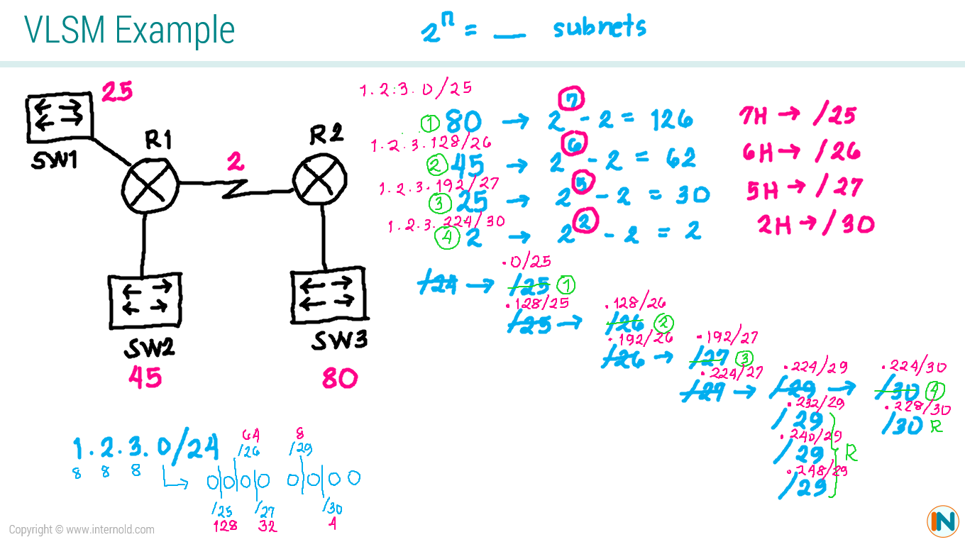
Practice Labs
Lab Challenge 1 - Static Routing
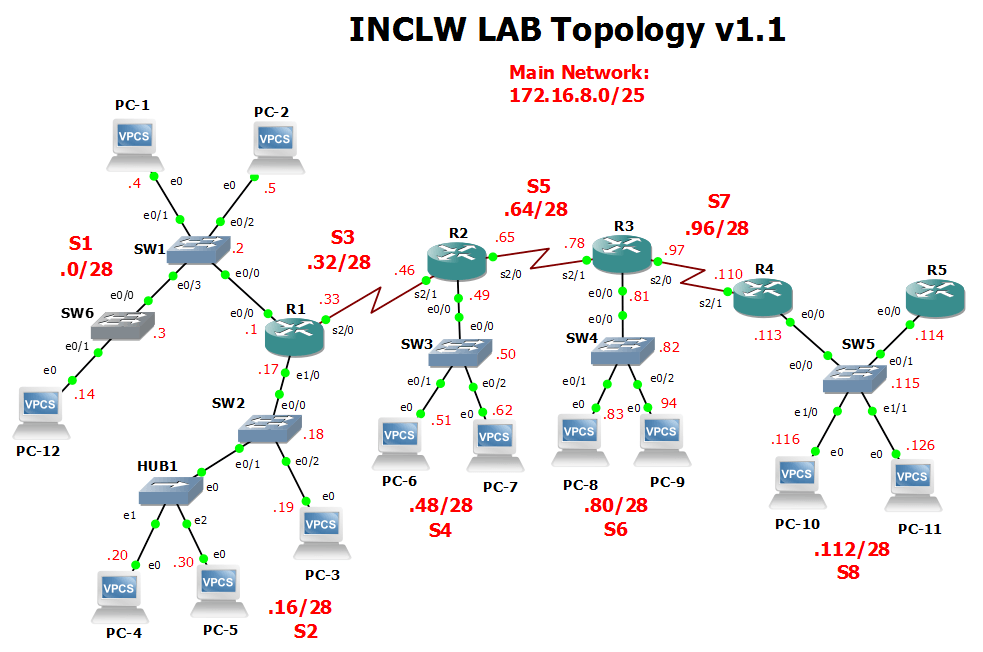

INCLW01 Week 3 Module
INTERNOLD NETWORKS CCNA LIVE WEBCLASS (INCLW)
week 3 module
Video Lessons
Video 1: Introduction
Video 2: DNS, ARP, and Ping
Video 3: Multiplexing Using Port Numbers
Video 4: Three-Way Handshake
Video 5: Reliability and Error Recovery
Video 6: Flow Control Using Windowing
Video 7: UDP
Video 8: Finding Web Using DNS
Video 9: Accessing The Catalyst Switch
Video 10: Learning MAC Address