

INCLW02 Week 1 Module
INTERNOLD NETWORKS CCNA LIVE WEBCLASS (INCLW)
week 1 module
Video Lessons
Video 1: Welcome and Introduction
Video 2: Perspective on Networking
Video 3: TCP/IP Networking Model
Video 4: History of TCP/IP Model
Video 5: TCP/IP Layers and Protocols
Video 6: TCP/IP Application & Transport Layer
Video 7: TCP/IP Network Layer
Video 8: TCP/IP Link Layer
Video 9: OSI Layer Overview
Video 10: OSI Layer Protocols and Data Encapsulation
Video 11: SOHO and Enterprise LANs
Video 12: Ethernet Physical and Data Link Standards
Video 13: Building Physical Ethernet Networks
Video 14: MAC Address
Video 15: Unicast Address + EtherType
Video 16: Full and Half Duplex
Video 17: Error Detection and Collision
Text Resources
Practice Quizzes
No results have been returned for your Query. Please edit the query for content to display.

Template Lesson
INTERNOLD NETWORKS CCNA LIVE WEBCLASS (INCLW)
Title Here
Contents
H1 Header
This is a paragraph
DHCP and IP Networking on Hosts
INTERNOLD NETWORKS CCNA LIVE WEBCLASS (INCLW)
DHCP and IP Networking on Hosts
Contents
DHCP and IP Networking on Hosts
In the world of TCP/IP, the word host refers to any device with an IP address: your phone, your tablet, a PC, a router, a switch—any device that uses IP to provide a service or just needs an IP address to be managed. The term host includes some less-obvious devices as well: the electronic advertising video screen at the mall, your electrical power meter that uses the same technology as mobile phones to submit your electrical usage information for billing, your new car.
No matter the type of host, any host that uses IPv4 needs four IPv4 settings to work properly:
IP address
Subnet mask
Default routersDNS server IP addresses
This last chapter in this part of the book completes the discussion of how to build a basic IPv4 network by focusing on the IPv4 settings on hosts. In particular, this chapter begins by discussing how a host can dynamically learn these four settings using the Dynamic Host Configuration Protocol (DHCP). The middle section of the chapter then discusses some tips for how to verify that a host has all four of these IPv4 settings. The third and final section takes a brief tangent to summarize and further explain the differences in the three main types of IPv4 addresses: unicast, broadcast, and multicast.
Implementing and Troubleshooting DHCP
Dynamic Host Configuration Protocol (DHCP) is one of the most commonly used protocols in a TCP/IP network. The vast majority of hosts in a TCP/IP network are user devices, and the vast majority of user devices learn their IPv4 settings using DHCP.
Using DHCP has several advantages over the other option of manually configuring IPv4 settings. The configuration of host IP settings sits in a DHCP server, with each client learning these settings using DHCP messages. As a result, the host IP configuration is controlled by the IT staff, rather than on local configuration on each host, resulting in fewer user errors. DHCP allows both the permanent assignment of host addresses, but more commonly, DHCP assigns a temporary lease of IP addresses. With these leases, the DHCP server can reclaim IP addresses when a device is removed from the network, making better use of the available addresses.
DHCP also enables mobility. For example, every time a user moves to a new location with a tablet computer—to a coffee shop, a client location, or back at the office—the user’s device can connect to another wireless LAN, use DHCP to lease a new IP address in that LAN, and begin working on the new network. Without DHCP, the user would have to ask for information about the local network and configure settings manually, with more than a few users making mistakes.
Although DHCP works automatically for user hosts, it does require some preparation from the network, with some configuration on routers. In some enterprise networks, that router configuration can be a single command on many of the router’s LAN interfaces (ip helper-address server-ip), which identifies the DHCP server by its IP address. In other cases, the router acts as the DHCP server. Regardless, the routers have some role to play.
This first major section of the chapter takes a complete tour of DHCP, from concept, to router configuration, verification, and troubleshooting.
DHCP Concepts
Sit back for a moment, and think about the role of DHCP for a host computer. The host acts as a DHCP client. As a DHCP client, the host begins with no IPv4 settings: no IPv4 address, no mask, no default router, and no DNS server IP addresses. But a DHCP client does have knowledge of the DHCP protocol, so the client can use that protocol to (a) discover a DHCP server and (b) request to lease an IPv4 address.
The DHCP process to lease an IP address uses the following four messages between the client and server. (Also, as a way to help remember the messages, note that the first letters spell DORA):
Discover: Sent by the DHCP client to find a willing DHCP server
Offer: Sent by a DHCP server to offer to lease to that client a specific IP address (and inform the client of its other parameters)
Request: Sent by the DHCP client to ask the server to lease the IPv4 address listed in the Offer message.
Acknowledgment: Sent by the DHCP server to assign the address, and to list the mask, default router, and DNS server IP addresses
DHCP clients, however, have a somewhat unique problem: they do not have an IP address yet, but they need to send IP packets. To make that work, DHCP messages make use of two special IPv4 addresses that allow a host that has no IP address to still be able to send and receive messages on the local subnet:
0.0.0.0: An address reserved for use as a source IPv4 address for hosts that do not yet have an IP address.
255.255.255.255: The local broadcast IP address. Packets sent to this destination address are broadcast on the local data link, but routers do not forward them.
To see how these addresses work, Figure 20-1 shows an example of the IP addresses used between a host (A) and a DHCP server on the same LAN. Host A, a client, sends a Discover message, with source IP address of 0.0.0.0 because host A does not have an IP address to use yet. Host A sends the packet to destination 255.255.255.255, which is sent in a LAN broadcast frame, reaching all hosts in the subnet. The client hopes that there is a DHCP server on the local subnet. Why? Packets sent to 255.255.255.255 only go to hosts in the local subnet; Router R1 will not forward this packet.

DHCP Discover and Offer
NOTE: Figure 20-1 shows one example of the addresses that can be used in a DHCP Request. This example shows details assuming the DHCP client chooses to use a DHCP option called the broadcast flag; all examples in this book assume the broadcast flag is used.
Now look at the Offer message sent back by the DHCP server. The server sets the destination IP address to 255.255.255.255 again. Why? Host A still does not have an IP address, so the server cannot send a packet directly to host A. So, the server sends the packet to “all local hosts in the subnet” address (255.255.255.255). (The packet is also encapsulated in an Ethernet broadcast frame.)
Note that all hosts in the subnet receive the Offer message. However, the original Discover message lists a number called the client ID, typically based on the host’s MAC address, that identifies the original host (host A in this case). As a result, host A knows that the Offer message is meant for host A. The rest of the hosts will receive the Offer message, but notice that the message lists another device’s DHCP client ID, so the rest of the hosts ignore the Offer message.
Supporting DHCP for Remote Subnets with DHCP Relay
Network engineers have a major design choice to make with DHCP: Do they put a DHCP server in every LAN subnet, or locate a DHCP server in a central site? The question is legitimate. Cisco routers can act as the DHCP server, so a distributed design could use the router at each site as the DHCP server. With a DHCP server in every subnet, as shown in Figure 20-1, the protocol flows stay local to each LAN.
However, a centralized DHCP server approach has advantages as well. In fact, some Cisco design documents suggest a centralized design as a best practice, in part because it allows for centralized control and configuration of all the IPv4 addresses assigned throughout the enterprise.
With a centralized DHCP server, those DHCP messages that flowed only on the local subnet in Figure 20-1 somehow need to flow over the IP network to the centralized DHCP server and back. To make that work, the routers connected to the remote LAN subnets need an interface subcommand: the ip helper-address server-ip command.
The ip helper-address server-ip subcommand tells the router to do the following for the messages coming in an interface, from a DHCP client:
1. Watch for incoming DHCP messages, with destination IP address 255.255.255.255.
2. Change that packet’s source IP address to the router’s incoming interface IP address.
3. Change that packet’s destination IP address to the address of the DHCP server (as configured in the ip helper-address command).
4. Route the packet to the DHCP server.
This command gets around the “do not route packets sent to 255.255.255.255” rule by changing the destination IP address. Once the destination has been set to match the DHCP server’s IP address, the network can route the packet to the server.
NOTE: This feature, by which a router relays DHCP messages by changing the IP addresses in the packet header, is called DHCP Relay.
Figure 20-2 shows an example of the process. Host A sits on the left, as a DHCP client. The DHCP server (172.16.2.11) sits on the right. R1 has an ip helper-address 172.16.2.11 command configured, under its G0/0 interface. At Step 1, Router R1 notices the incoming DHCP packet destined for 255.255.255.255. Step 2 shows the results of changing both the source and destination IP address, with R1 routing the packet.

IP Helper Address Effect
The router uses a similar process for the return DHCP messages from the server. First, for the return packet from the DHCP server, the server simply reverses the source and destination IP address of the packet received from the router (relay agent). For example, in Figure 20-2, the Discover message lists source IP address 172.16.1.1, so the server sends the Offer message back to destination IP address 172.16.1.1.
When a router receives a DHCP message, addressed to one of the router’s own IP addresses, the router realizes the packet might be part of the DHCP relay feature. When that happens, the DHCP relay agent (Router R1) needs to change the destination IP address, so that the real DHCP client (host A), which does not have an IP address yet, can receive and process the packet. Figure 20-3 shows one example of how these addresses work, when R1 receives the DHCP Offer message sent to R1’s own 172.16.1.1 address. R1 changes the packet’s destination to 255.255.255.255, and forwards it out G0/0, because the packet was destined to G0/0’s 172.16.1.1 IP address. As a result, all hosts in that LAN (including the DHCP client A) will receive the message.

IP Helper Address for the Offer Message Returned from the DHCP Server
Many enterprise networks use a centralized DHCP server, so the normal router configuration includes an ip helper-address command on every LAN interface/subinterface. With that standard configuration, user hosts off any router LAN interface can always reach the DHCP server and lease an IP address.
Information Stored at the DHCP Server
A DHCP server might sound like some large piece of hardware, sitting in a big locked room with lots of air conditioning to keep the hardware cool. However, like most servers, the server is actually software, running on some server OS. The DHCP server could be a piece of software downloaded for free and installed on an old PC. However, because the server needs to be available all the time, to support new DHCP clients, most companies install the software on a very stable and highly available data center, but the DHCP service is still created by software.
To be ready to answer DHCP clients, and to supply them with an IPv4 address and other information, the DHCP server (software) needs configuration. DHCP servers typically organize these IPv4 settings per subnet, because the information the server tells the client is usually the same for all hosts in the same subnet, but slightly different for different subnets. For example, IP addressing rules tell us that all hosts on the same subnet should use the same mask, but hosts in different subnets would have a different default gateway setting.
The following list shows the types of settings the DHCP server needs to know to support DHCP clients:
Subnet ID and mask: The DHCP server can use this information to know all addresses in the subnet. (The DHCP server knows to not lease the subnet ID or subnet broadcast address.)
Reserved (excluded) addresses: The server needs to know which addresses in the subnet to not lease. This list allows the engineer to reserve addresses to be used as static IP addresses. For example, most router and switch IP addresses, server addresses, and addresses of most anything other than user devices use a statically assigned IP address. Most of the time, engineers use the same convention for all subnets, either reserving the lowest IP addresses in all subnets, or reserving the highest IP addresses in all subnets.
Default router(s): This is the IP address of the router on that subnet.
DNS IP address(es): This is a list of DNS server IP addresses.
Figure 20-4 shows the concept behind the preconfiguration on a DHCP server for two LAN-based subnets, 172.16.1.0/24 and 172.16.2.0/24. The DHCP server sits on the right. For each subnet, the server defines all the items in the list. In this case, the configuration reserves the lowest IP addresses in the subnet to be used as static addresses.

Preconfiguration on a DHCP Server
The configuration can list other parameters as well. For example, it can set the time limit for leasing an IP address. The server leases an address for a time (usually a number of days), and then the client can ask to renew the lease. If the client does not renew, the server can reclaim the IP address and put it back in the pool of available IP addresses. The server configuration sets the maximum time for the lease.
DHCP uses three allocation modes, based on small differences in the configuration at the DHCP server. Dynamic allocation refers to the DHCP mechanisms and configuration described throughout this chapter. Another method, automatic allocation, sets the DHCP lease time to infinite. As a result, once the server chooses an address from the pool and assigns the IP address to a client, the IP address remains with that same client indefinitely. A third mode, static allocation, preconfigures the specific IP address for a client based on the client’s MAC address. That specific client is the only client that then uses the IP address. (Note that this chapter shows examples and configuration for dynamic allocation only.)
Of note, the exam topics mention one other configuration DHCP server setting for a value that can be passed to DHCP clients—the IP address of a Trivial File Transfer Protocol (TFTP) server. TFTP servers provide a basic means of storing files that can then be transferred to a client host. As it turns out, Cisco IP phones rely on TFTP to retrieve several configuration files when the phone initializes. DHCP plays a key role by supplying the IP address of the TFTP server that the phones should use.
DHCP Server Configuration on Routers
A quick Google search on “DHCP server products” reveals that many companies offer DHCP server software. Cisco routers (and some Cisco switches) can also act as a DHCP server with just a little added configuration.
Configuring a Cisco router to act as a DHCP server uses a new configuration concept, one per subnet, called a DHCP pool. All the per-subnet settings go into a per-subnet DHCP pool. The only DHCP command that sits outside the pool is the command that defines the list of addresses excluded from being leased by DHCP. The Cisco IOS DHCP server configuration steps are as follows:
Step 1. Use the ip dhcp excluded-address first last command in global configuration mode to list addresses that should be excluded (that is, not leased by DHCP).
Step 2. Use the ip dhcp pool name command in global configuration mode to both create a DHCP pool for a subnet and to navigate into DHCP pool configuration mode. Then also:
A. Use the network subnet-ID mask or network subnet-ID prefix-length command in DHCP pool configuration mode to define the subnet for this pool.
B. Use the default-router address1 address2... command in DHCP pool configuration mode to define default router IP address(es) in that subnet.
C. Use the dns-server address1 address2... command in DHCP pool configuration mode to define the list of DNS server IP addresses used by hosts in this subnet.
D. Use the lease days hours minutes command in DHCP pool configuration mode to define the length of the lease, in days, hours, and minutes
E. Use the domain-name name command in DHCP pool configuration mode to define the DNS domain name.
F. Use the next-server ip-address command in DHCP pool configuration mode to define the TFTP server IP address used by any hosts (like phones) that need a TFTP server.
Of course, an example can help, particularly with so many configuration commands required. Figure 20-5 shows the organization of the configuration, while sticking to pseudocode rather than the specific configuration commands. (Upcoming Example 20-1 shows a matching configuration.) Note that for each of the two LAN subnets, there is a global command to exclude addresses, and then a group of settings for each of two different DHCP pools.

DHCP Server Configuration Pseudocode
Example 20-1 R2 as a DHCP Server Per the Concepts in Figure 20-5

R2 as a DHCP Server Per the Concepts in Figure 20-5
Focus on subnet 172.16.1.0/24 for a moment: the subnet configured as pool subnet-left. The subnet ID and mask match the subnet ID chosen for that subnet. Then, the global ip dhcp excluded-address command, just above, reserves 172.16.1.1 through 172.16.1.50, so that this DHCP server will not lease these addresses. The server will automatically exclude the subnet ID (172.16.1.0) as well, so this DHCP server will begin leasing IP addresses starting with the .51 address.
Now look at the details for subnet-right. It uses a DHCP pool network command with a prefix style mask. It defines the same DNS server, as does the pool for the other subnet, but a different default router setting, because, of course, the default router in each subnet is different. This pool includes a lease time of 1:02:03 (1 day, 2 hours, and 3 minutes) just as an example.
Also note that both subnets list a TFTP server IP address of the Unified Communications Manager (UCM) server with the next-server command. In most cases, you would find this setting in the pools for subnets in which phones reside.
Finally, note that configuring a router as a DHCP server does not remove the need for the ip helper-address command. If DHCP clients still exist on LANs that do not have a DHCP server, then the routers connected to those LANs still need the ip helper-address command. For example, in Figure 20-5, R1 would still need the ip helper-address command on its LAN interface. R2 would not need the command on its LAN interface, because R2 could service those requests, rather than needing to forward the DHCP messages to some other server.
IOS DHCP Server Verification
The IOS DHCP server function has several different show commands. These three commands list most of the details:
show ip dhcp binding: Lists state information about each IP address currently leased to a client
show ip dhcp pool [poolname]: Lists the configured range of IP addresses, plus statistics for the number of currently leased addresses and the high-water mark for leases from each pool
show ip dhcp server statistics: Lists DHCP server statistics
Example 20-2 shows sample output from two of these commands, based on the configuration from Figure 20-5 and Example 20-1. In this case, the DHCP server leased one IP address from each of the pools, one for host A, and one for host B, as shown in the highlighted portions of the output.
Example 20-2 Verifying Current Operation of a Router-Based DHCP Server

Verifying Current Operation of a Router-Based DHCP Server
Note that the output in Example 20-2 does not happen to list the excluded addresses, but it does show the effects. The addresses assigned to the clients end with .51 (host A, subnet 172.16.1.0) and .101 (host B, subnet 172.16.2.0), proving that the server did exclude the addresses as shown in the configuration in Example 20-1. The server avoided the .1 through .50 addresses in subnet 172.16.1.0, and the .1 through .100 addresses in subnet 172.16.2.0.
NOTE: The DHCP server keeps status (state) information about each DHCP client that leases an address. Specifically, it remembers the DHCP client ID, and the IP address leased to the client. As a result, an IPv4 DHCP server can be considered to be a stateful DHCP server. This description will be useful when reading about DHCP for IPv6 in Chapter 31, “Implementing IPv6 Addressing on Hosts.”
Troubleshooting DHCP Services
Chapter 19, “Learning IPv4 Routes with RIPv2,” closed with a section about troubleshooting RIPv2. That section makes the point that to be ready for Simlet questions in particular, you have to be ready to predict what symptoms would occur when the network was misconfigured in particular ways. This next section takes a similar approach, pointing out the most typical issues that could be introduced through incorrect or missing configuration, and then discussing what symptoms should happen and how to recognize those problems.
This section begins with a typical look at configuration mistakes and the symptoms that occur with those mistakes. In particular, this section looks at problems with the relay agent’s helper address as well as the IOS DHCP server configuration. This section then looks at non-DHCP problems related to that data plane, breaking the problem into issues between the client and relay agent, and between the relay agent and DHCP server. The final section takes a short look at how a DHCP server prevents duplicate IP addresses between hosts that use static IP addresses and those that use DHCP.
DHCP Relay Agent Configuration Mistakes and Symptoms
One configuration mistake that prevents DHCP client from leasing an IP address is the misconfiguration or the omission of the ip helper-address interface subcommand on the router acting as the DHCP relay agent. The relay agent takes the incoming DHCP message, changes the destination address of the packet to be the address on the ip helper-address address command, and forwards the packet to that address. If the command is missing, the router does not attempt to forward the DHCP messages at all; if it is incorrect, the relay agent forwards the DHCP packets, but they never arrive at the actual DHCP server.
The main problem symptom in this case is the failure of a DHCP client to lease an address. If you can identify a client that has a problem, and you know what VLAN or subnet in which that host resides, you can then work to identify any routers connected to that subnet, to find and correct the ip helper-address subcommands.
Beyond that step, this list summarizes a few other related points.
The DHCP relay agent feature is needed on interfaces only if the DHCP server is on a different subnet; it is not needed if the DHCP server is on the same subnet as the client.
On routers with VLAN trunks (with a router-on-a-stick [ROAS] subinterface configuration), the subinterfaces also need an ip helper-address command (assuming they meet the first criteria in this list).
If an exam question does not allow you to look at the configuration, use the show ip interface [type number] command to view the ip helper-address setting on an interface.
About that last point, Example 20-3 shows an example of the show ip interface g0/0 command. In this case, the interface has been configured with the ip helper-address 172.16.2.11 command; the show command output basically restates that fact. (The configuration matches the earlier examples surrounding Figures 20-2 and 20-3 for Router R1.) Note that if there were no ip helper-address configured on the interface, the text would instead read “Helper address is not set.”
Example 20-3 Listing the Current Helper Address Setting with show ip interface

Listing the Current Helper Address Setting with show ip interface
IOS DHCP Server Configuration Mistakes and Symptoms
When using an IOS DHCP server, from a troubleshooting perspective, break issues into two broad categories: those that prevent DHCP clients from leasing an address, and those that allow the lease but provide incorrect settings to the client.
First, the primary configuration mistake that causes a failure in the DHCP lease process is the misconfiguration of the network command. The problem revolves around these key facts:
The packet from the relay agent to the DHCP server uses the relay agent’s interface IP address as the source IP address in the forwarded DHCP message. (See Figure 20-2 for a reminder.)
The DHCP server compares that source IP address in the received DHCP packet to the network commands in its DHCP pools to find the right pool.
Each network subnet mask command implies a range of addresses, just like any other IP network or subnet shown with a subnet mask.
If the source IP address of the packet is not in the range of addresses implied by any network command in all the pools, the DHCP server has no pool to use for that request. The DHCP server does not know how to respond, so it does not reply at all.
As an example of that failure, consider the configuration shown in Figure 20-6. The left side shows the configuration on R1, a DHCP relay agent that has two interfaces configured with the ip helper-address 172.16.2.11 command. The DHCP server configuration on the right lists two pools, intended as one pool for each subnet off Router R1. However, the network 172.16.3.0 /25 command implies an address range of 172.16.3.0 to 172.16.3.127, and the relay agent’s interface address of 172.16.3.254 is not within that range of numbers. The solution would be to correct the DHCP server’s network command to use a /24 mask.

An Example Misconfiguration of a DHCP Pool network Command
NOTE: The ip helper-address configuration on the left is correct. The figure uses a ROAS configuration here just to reinforce the comment in the earlier section that ROAS subinterfaces also need an ip helper-address subcommand.
While you ultimately need to find this kind of problem and fix the configuration, on the exam you need to be ready to discover the root cause based on symptoms and show commands as well. So, when troubleshooting DHCP issues, and the client fails to lease an address, look at the IOS DHCP server’s network commands. Calculate the range of IP addresses as if that command were defining a subnet. Then compare that range of addresses by the network command in each pool to the interface addresses on the DHCP relay agent routers. Every relay agent interface (that is, every interface with an ip helper-address command configured) should be included in a pool defined at the IOS DHCP server.
The DHCP server can also be misconfigured in a way that allows the lease of an address, but then causes other problems. If the lease process works, but the rest of the parameters given to the client are incorrect or missing, the client could operate, but operate poorly. This list summarizes the kinds of mistakes and the resulting symptoms:
With the DNS server IP addresses incorrectly configured on the server (or omitted), hosts would fail to resolve hostnames into their associated IP addresses.
With the default gateway IP address incorrectly configured on the server (or omitted), hosts could not communicate outside the local subnet.
With the TFTP server IP address incorrectly configured (or omitted), an IP phone would fail to correctly load its configuration.
Chapter 24, “Troubleshooting IPv4 Routing,” discusses host troubleshooting in more depth, including these issues.
IP Connectivity from DHCP Relay Agent to DHCP Server
For the DHCP process to work with a centralized server, IP broadcast packets must flow between the client and relay agent, and IP unicast packets must flow between the relay agent and the DHCP server. Any problem that prevents the flow of these packets also prevents DHCP from working.
For perspective, consider the topology in Figure 20-7, which again shows the relay agent on the left and the DHCP server on the right. The server uses IP address 172.16.2.11, and the relay agent uses interface address 172.16.1.1. Any failure that prevents the flow of IP packets between those two IP addresses would prevent host A from leasing an IP address.

Addresses Used between Relay Agent and Server
This chapter does not attempt to work through IP troubleshooting. However, two upcoming chapters explain two useful tools (extended ping and traceroute commands, Chapter 23, “IPv4 Troubleshooting Tools,”) and then describe how to troubleshoot DHCP connectivity in particular (“DHCP Issues” in Chapter 24. For now, remember the IP addresses used on the packets between the relay agent and server, and know that you may need to troubleshoot IP routing to ensure those packets can be delivered.
LAN Connectivity Between the DHCP Client and Relay Agent
Back in Figures 20-1, 20-2, and 20-3, you saw that the DHCP messages on the same LAN as the DHCP client all showed a destination IP address of 255.255.255.255. What does that really mean? When a packet uses this 255.255.255.255 address:
The address is called the local broadcast address.
Packets sent to this address are not forwarded as-is by routers.
On a LAN, the sender of an IP local broadcast packet encapsulates these IP packets in an Ethernet frame with an Ethernet broadcast destination address (FFFF.FFFF.FFFF), so the LAN broadcasts the frame.
As a result of the logic in these steps, the broadcast DHCP messages can easily flow between the client and router, as long as the LAN works. Chapter 12, “Troubleshooting Ethernet LANs,” discusses how to troubleshoot the LAN.
Summary of DHCP Troubleshooting
In summary, as a study tool, the following list summarizes the key troubleshooting ideas from this chapter:
Step 1. If using a centralized DHCP server, at least one router on each remote subnet that has DHCP clients must act as DHCP relay agent, and have a correctly configured ip helper-address address subcommand on the interface connected to that subnet.
Step 2. If using a centralized IOS DHCP server, make sure the DHCP pools’ network commands match the entire network’s list of router interfaces that have an ip helper-address command pointing to this DHCP server.
Step 3. Troubleshoot for any IP connectivity issues between the DHCP relay agent and the DHCP server, using the relay agent interface IP address and the server IP address as the source and destination of the packets.
Step 4. Troubleshoot for any LAN issues between the DHCP client and the DHCP relay agent.
Also, as one final note about DHCP in the real world, DHCP might seem dangerous at this point, with all the focus on potential problems in this section, combined with the importance of DHCP and its use by most end user devices. However, DHCP has some great availability features. First, most DHCP servers set their lease times for at least a few days, often a week, or maybe longer. Combined with that, the DHCP protocol has several processes through which the client reconfirms the existing lease with the server, and releases the same IP address in advance of the expiration of the lease. Clients do not simply wait until the moment the lease would expire to then contact the DHCP server, hoping it is available. So the network can have outages, and DHCP clients that have already leased an address can continue to work without any problem.
Detecting Conflicts with Offered Versus Used Addresses
Beyond troubleshooting the types of problems that would prevent DHCP from working, the IOS DHCP server tries to prevent another type of problem: assigning IP addresses with DHCP when another host tries to statically configure that same IP address. Although the DHCP server configuration clearly lists the addresses in the pool, plus those to be excluded from the pool, hosts can still statically configure addresses from the range inside the DHCP pool. In other words, no protocols prevent a host from statically configuring and using an IP address from within the range of addresses used by the DHCP server.
Knowing that some host might have statically configured an address from within the range of addresses in the DHCP pool, both DHCP servers and clients try to detect such problems, called conflicts, before the client uses a newly leased address.
DHCP servers detect conflicts by using pings. Before offering a new IP address to a client, the DHCP server first pings the address. If the server receives a response to the ping, some other host must already be using the address, which lets the server know a conflict exists. The server notes that particular address as being in conflict, and the server does not offer the address, moving on to the next address in the pool.
The DHCP client can also detect conflicts, but instead of using ping, it uses ARP. In the client case, when the DHCP client receives from the DHCP server an offer to use a particular IP address, the client sends an Address Resolution Protocol (ARP) request for that address. If another host replies, the DHCP client has found a conflict.
Example 20-4 lists output from the router-based DHCP server on R2, after host B detected a conflict using ARP. Behind the scenes, host B used DHCP to request a lease, with the process working normally until host B used ARP and found some other device already used 172.16.2.102. At that point, host B then sent a DHCP message back to the server, rejecting the use of address 172.16.2.102. The example shows the router’s log message related to host B’s discovery of the conflict, and a show command that lists all conflicted addresses.
Example 20-4 Displaying Information About DHCP Conflicts in IOS

Edit your caption text here
The show ip dhcp conflict command lists the method through which the server added each address to the conflict list: either gratuitous ARP, as detected by the client, or ping, as detected by the server. The server avoids offering these conflicted addresses to any future clients, until the engineer uses the clear ip dhcp conflict command to clear the list.
Verifying Host IPv4 Settings
Some hosts use DHCP to learn their IPv4 settings. Others manually set all their settings. Other hosts actually allow you to make some settings manually, and learn other settings with DHCP.
Regardless of how a given host builds its IPv4 configuration, that host will either work, or have problems. And if it has problems, someone needs to be ready and able to jump in and help solve the problem. On hosts, that means someone needs to be able to find the IPv4 settings, make sure they are correct, and troubleshoot problems related to the host IP settings.
This short section brushes the surface of how to verify IPv4 settings on hosts. This section touches on each of the settings, showing some host commands used to confirm each setting, as well as giving a few related hints on how to confirm if it is working or not.
IP Address and Mask Configuration
Most every OS in the world—certainly the more common OSs people work with every day—have a fairly easy-to-reach window that lists most if not all the IPv4 settings in one place. For example, Figure 20-8 shows the Network configuration screen from a user host OS (Mac OS X in this case), with all the IPv4 settings. This particular example shows the big four settings: address, mask, router, and DNS.

IP Address, Mask, and Default Router Settings on Mac OS
However, beyond these windows into the graphical user interface (GUI) of any OS, most OSs have a variety of networking commands available from a command line. Interestingly, some of the commands are the same across many different OSs, even between Microsoft Windows versions and other OSs.
For example, to verify the IP address, mask, default router, and other settings, OSs typically support either the ipconfig (Windows) or ifconfig (Linux and Mac OS) commands. Both commands have several options that can be seen by adding a -? to the end. Example 20-5 shows a sample from a Windows PC.
Example 20-5 ipconfig /all (Windows)

ipconfig /all (Windows)
Name Resolution with DNS
The Domain Name System (DNS) defines a protocol as well as a worldwide system of servers that use DNS. While incredibly useful—it might be one of the single most important protocols in the world of TCP/IP—DNS does not require attention from the routers and switches between the user devices and the DNS servers. This short section explains why, but shows you a few router commands related to DNS that might be handy anyway.
Inside a single enterprise, the company uses a couple of redundant DNS servers, each of which can resolve any host names for any hosts inside the company. Figure 20-9 shows an example using a single company, with a client on the left using the DNS server at the top of the figure. Step 1 shows the DNS Request message, asking the DNS server to resolve name “Server1” into its corresponding IP address. The DNS server sends back a DNS Reply, listing the IP address. Finally, at Step 3, the client can send a packet to 10.1.2.3, the address used by Server1.

Host Resolves Name to IP Address Before Sending Packet to Server1
Now stop for a moment, and focus on the To: part of the three messages. Each packet has a known unicast destination address. The routers in the TCP/IP network can simply forward those packets. No need for any special configuration, no need for a command and function like the ip helper-address command used with DHCP. In short, the routers and switches have no extra work to do, and no extra configuration required, to support DNS between a host and the DNS servers.
Default Routers
As discussed in some detail back in Chapter 18, IPv4 host routing logic reduces to a basic two-part choice. For packets destined for a host in the same subnet, the local host sends the packet directly, ignoring any routers. For packets destined for a host in a different subnet, the local host next sends the packet to its default gateway (also known as the default router), expecting that router to forward the packet.
Interestingly, a couple of simple errors can occur between any LAN-based host and their default router. For a LAN-based host’s default router setting to work, the following must be true:
The host link to the LAN and the default router link to the LAN must be in the same VLAN.
The host and default router IP addresses must be in the same subnet.
The host default router setting must refer to the same IP address configured on the router. (In other words, if the host claims the default router is 10.1.1.1, make sure the router interface IP address is not 10.1.1.2.)
The LAN switches must not discard the frame because of the port security configuration.
All of the preceding settings and choices can be mismatched between a host and the default router. On the router, the settings can be checked with the usual CLI commands: show interfaces, show ip interface brief, show protocols, and show running-config. On the switch, to check the VLAN assignments, use show interfaces status, show vlan, and show interfaces switchport.
On the host, the methods to check the default router setting of course differ depending on the OS. A look at the settings using the GUI simply lists the default router. However, a common command on most user host OSs is the netstat -rn command, which lists the default gateway as the route for either destination 0.0.0.0 or as default. Example 20-6 shows a netstat -rn command from a Mac, with the default router setting highlighted.
Example 20-6 netstat -rn Command (Mac OS X)

netstat -rn Command (Mac OS X)
Another good step to take to verify the default router is to find out whether ARP works for the default router. For example, host A in Figure 20-10, when sending packets to host D, in the same subnet, will send the packet directly to host D. So, host A will first need an ARP entry for host D. Similarly, before sending a packet to server B, which sits on another subnet, host A will need an ARP entry for R1’s MAC address.

Host IP and MAC Addresses in the Next Two ARP Examples
The arp -a command happens to be another common command on many user OSs. Example 20-7 shows host A’s ARP table after host A successfully sent a packet to both server B and host D. Note that server B’s IP address of 172.16.2.9 is not listed, because the ARP table lists IP addresses for IP addresses on the same subnet, and not those on remote subnets.
Example 20-7 ARP Table on Host A (Windows)

ARP Table on Host A (Windows)
Routers also need to keep an ARP table, so they can encapsulate IP packets into LAN frames. Example 20-8 shows the output of the show arp command on Router R1, which lists an entry for host A (172.16.1.9), and for the router itself (172.16.1.1). (Note that hosts typically do not list their own IP addresses in their own ARP cache, but the Cisco router ARP cache does.)
Example 20-8 ARP Table on Router R1

ARP Table on Router R1
IPv4 Address Types
The IPv4 address space includes three major categories of addresses: unicast, broadcast, and multicast. For the current exam, Cisco lists one exam topic that asks you to compare and contrast these address types. To help you make those comparisons, this section explains multicast addressing, while pulling together the key ideas about unicast and broadcast IP addresses that have already been introduced, to pull the ideas together.
You may be wondering why this topic about IPv4 address types sits at the end of a chapter about DHCP and IP networking on hosts. Honestly, I could have put this topic in several chapters. The main reason it is here is that you have already seen the IP broadcast addresses in action, including the 255.255.255.255 local broadcast as shown in this chapter.
Review of Unicast (Class A, B, and C) IP Addresses
Unicast IP addresses are those Class A, B, and C IP addresses assigned to hosts, router interfaces, and other networking devices. Because most discussions about IP addressing refer to unicast IP addresses, most of us just refer to them as IP addresses, and leave out the word unicast.
Just to be complete and define the concept, unicast addresses identify one interface on one device to IP. Just like your postal address gives the post office an address to use to send letters to your one specific house or apartment, a unicast IP address gives the IP network an address to use to send packets to one specific host. However, with IP, instead of addressing the device, unicast addresses identify individual interfaces. For example:
A router with four LAN interfaces, and two WAN interfaces, have six unicast addresses, each in a different subnet, one for each interface.
A PC with both an Ethernet network interface card (NIC) and a wireless NIC would have two unicast IPv4 addresses, one for each interface.
IP Broadcast Addresses
Broadcast IPv4 addresses give IP a way to send one packet that the network delivers to multiple hosts. IPv4 defines several types of broadcast addresses, with each type being used to reach a different set of hosts. These different broadcast IP addresses give different overhead protocols like DHCP the ability to efficiently reach all hosts in a specific part of the network. The following list reviews the three IP broadcast address types:
Local broadcast address: 255.255.255.255. Used to send a packet on a local subnet, knowing that routers will not forward the packet as is. Also called a limited broadcast.
Subnet broadcast address: One reserved address for each subnet, namely the numerically highest number in the subnet, as discussed in Chapter 15, “Analyzing Subnet Masks.” A packet sent to a subnet broadcast address can be routed to the router connected to that subnet, and then sent as a data link broadcast to all hosts in that one subnet. Also called an all-hosts broadcast to emphasize that all hosts in a subnet are reached, and also called a directed broadcast.
Network broadcast address: One reserved address for each classful network, namely the numerically highest number in the network. Used to send one packet to all hosts in that one network. Also called an all-subnets broadcast, referring to the fact that the packet reaches all subnets in a network.
This chapter has already shown how a local broadcast works, sending the message over the same subnet in which it was first transmitted, but no further. However, the other two types are a little more interesting.
Subnet and network broadcasts provide a way to send packets to all hosts in a subnet or network (respectively) while reducing waste. For instance, with a subnet broadcast, routers forward the packet just like any other IP packet going to that subnet. When that packet arrives at the router connected to that subnet, the last router then encapsulates the packet in a LAN broadcast, so that all hosts receive a copy. Figure 20-11 shows the idea.

Example of a Subnet Broadcast to 10.1.1.255
The figure shows two key points. R1 does not flood or broadcast the frame to all other routers, instead routing it to the next router (R2 in this case) so that the packet reaches subnet 10.1.1.0/24. R2, connected to subnet 10.1.1.0/24, forwards the packet onto the LAN, but encapsulates the packet in an Ethernet broadcast frame, so that it reaches all hosts in the subnet.
The figure shows the intended use of the subnet broadcast address; however, it presents a security issue today. Many attacks start with a ping to subnet broadcast addresses, hoping to get many hosts to reply. Cisco changed the IOS default many years ago to disable the forwarding of subnet broadcasts onto a connected subnet (that is, it disables Step 3 in Figure 20-11). That default setting is based on the no ip directed-broadcast interface subcommand.
A network broadcast packet (a packet with a network broadcast address as the destination) works in a similar way. To reach all subnets, however, the routers create copies of the packet and flood it so it reaches all subnets inside the classful network. On any LAN interfaces, the packet is forwarded in a LAN broadcast, just as shown in Step 3 of Figure 20-11.
IPv4 Multicast Addresses (Class D Addresses)
Multicast IP addresses and the related protocols help solve a similar problem as compared to broadcast addresses, but mainly for applications, and without the same security issues experienced by broadcast addresses. To see how it works, consider this example. A video application may be designed to show live video feeds. If 10 people at the same remote site in the same subnet want to watch the same video at the same time, the application could be designed so that the application sent the same video data 10 times, once to each client in the same subnet. An application designed to use Class D multicast addresses could send 1 packet, which the routers would route across the WAN, and then deliver a copy to all 10 hosts in the destination subnet.
When using multicast, all the hosts still use their individual unicast IP address for their normal traffic, while also using the same multicast IPv4 address for the multicast application. Any server or client that happens to use an application designed to take advantage of IP multicast then also uses the Class D multicast addresses that the application chooses to use. You can think of a Class D address more as a multicast group—in fact, it is often called that—because hosts join the group so that they can receive the packets sent by the multicast application.
Class D addresses begin with a first octet of between 224 and 239, with some ranges reserved for various purposes. Much of the Class D address space is set aside for a company to deploy one of these multicast applications, and then pick an address from the Class D range, and configure it to be used by a multicast application.
As an example, imagine the video application uses Class D address 226.1.1.1. Figure 20-12 illustrates the process by which the application at the server on the left sends one multicast packet with destination address 226.1.1.1. Note that for this process to work, the hosts with * beside them registered with their local routers to notify the routers that the host wants to receive packets destined to multicast address 226.1.1.1. When the action in this figure begins, the routers collectively know which subnets have hosts that want a copy of multicasts sent to 226.1.1.1, and which subnets do not.

Example of a Multicast Packet Flow for Three Registered Hosts
Following the steps in the figure:
1. The server on the left generates and sends a multicast packet.
2. Router R1 replicates the packet to send a copy to both R2...
3. ...and to R3. R1 does not replicate and send a copy to R4, because there are no hosts near R4 listening for packets sent to 226.1.1.1.
4. R2 processes the multicast packet received from R1, and because of the earlier host registration process, R2 knows that at least one host off both its LAN interfaces are listening for packets sent to 226.1.1.1. R2 therefore forwards a copy of the packet out each of its LAN interfaces.
5. R3 receives the multicast packet from R1, and uses the same kind of logic as R2. However, R3 knows from the earlier host registration process that only one of its LAN interfaces connects to a subnet with hosts listening for packets sent to 226.1.1.1, so R3 forwards a copy of the packet out that one interface only.
As you can see from this example, the server sent one packet and the routers replicated the packet so it reached all the correct locations in the network.
As another comparison between unicast and multicast addresses, note that multicast addresses may be used as destination IP addresses only, whereas unicast addresses may be used as both the destination and source address. For instance, consider the packets in the example shown in Figure 20-12. All those packets flow from one host, so the packet uses a unicast IP address of that host’s unicast IP address.
Finally, to complete one more comparison between unicast IP addressing and multicast IP addressing, think about that last hop router in the example shown in Figure 20-11. If a router such as R2 or R3 had forwarded a unicast IP packet, the router would look in its ARP cache to find the unicast IP address for the destination in that connected subnets, and the associated unicast MAC address. That will not work when forwarding a multicast packet with a multicast (Class D) destination IP address.
To encapsulate a multicast IP packet over an Ethernet LAN, IP multicast calculates the destination MAC address with a simple process. The process copies the last 23 bits of the IP address behind a reserved 25-bit prefix to form the 48-bit destination MAC address. The resulting MAC address, called a multicast MAC address, begins with hex 01005E. So, the multicast IP packet, encapsulated in the multicast Ethernet frame, is forwarded out the router interface onto the LAN. At that point, the switches take one of the following approaches to forwarding the frame so that all hosts who want a copy of the frame get a copy:
Flood the multicast frame as if it were a broadcast
Use other Ethernet multicast features that flood the frame only to those same devices that registered to receive a copy
If you feel like these few pages probably left out some detail; indeed, several books have been written about IP multicast all to itself. The topic is indeed large. For this book’s purposes, know the main comparison points with unicast addressing. Multicast addressing gives applications that need to communicate the same data at the same time to multiple hosts a much more efficient way to do that. If the application is written to make use of IP multicast, the application can consume much less traffic in the network, as compared to using unicast IP addresses and sending every host a copy of the packet.
Comparing and Contrasting IP Address Types
The last few pages reviewed unicast and broadcast addresses, and explained the core concepts behind IP multicast addresses. Table 20-2 summarizes the key comparison points mentioned throughout this section for convenient study.

Comparisons of Unicast, Broadcast, and Multicast IP Addresses
Troubleshooting IPv4 Routing
INTERNOLD NETWORKS CCNA LIVE WEBCLASS (INCLW)
Troubleshooting IPv4 Routing
Contents
Troubleshooting IPv4 Routing
By this point in the book, you have learned a lot about IPv4 addressing, subnetting, and routing. The four chapters in Part IV explained the basics of IPv4 addressing. Then Part V showed how to implement simple IPv4 networks with routers, showing how to configure the control plane so that routers learned the correct routes. That part also linked in how hosts work along with their nearby default router. And now Part VI has added more detail to your knowledge, with more advanced IP addressing and subnetting topics, and with troubleshooting tools in the previous chapter.
This chapter has one obvious goal and one not-so-obvious goal. The obvious goal is to discuss troubleshooting of how IPv4 routing works. This chapter pulls together the ideas about the IPv4 data plane that have already been discussed in Parts IV, V, and VI. However, this chapter takes a troubleshooting approach, discussing what could go wrong and what the symptoms would be if they did go wrong.
This chapter also reviews several topics related to the IPv4 data plane all in one chapter. This book contains a lot of content about IPv4, and reading through the content in this chapter can help you realize which topics you already understand well, and which topics you did not quite master yet. To that end, this chapter’s second big goal is to give you a chance to identify weaker areas and to strengthen your understanding, before moving on to the final third or so of this book.
This chapter breaks the topics into two major sections. The first major section focuses on issues between a host and its default router. The second major section then looks at issues that prevent routers from forwarding packets.
Problems Between the Host and the Default Router
Imagine that you work as a customer support representative (CSR) fielding calls from users about problems. A user left a message stating that he couldn’t connect to a server. You could not reach him when you called back, so you did a series of pings from that host’s default router. At the end of those pings, you think the problem exists somewhere between the user’s device and the default router—for instance, between Router R1 and host A, as shown in Figure 24-1.

Figure 24-1 Focus of the Discussions in This Section of the Chapter
This first major section of the chapter focuses on problems that can occur on hosts, their default routers, and between the two. To begin, this section looks at the host itself, and its four IPv4 settings, as listed in the figure. Following that, the discussion moves to the default router, with focus on the LAN interface, and the settings that must work for the router to serve as a host’s default router.
Root Causes Based on a Host’s IPv4 Settings
A typical IPv4 host gets its four key IPv4 settings in one of two ways: either through static configuration or by using Dynamic Host Configuration Protocol (DHCP). In both cases, the settings can actually be incorrect. Clearly, any static settings can be set to a wrong number just through human error when typing the values. More surprising is the fact that the DHCP can set the wrong values: The DHCP process can work, but with incorrect values configured at the DHCP server, the host can actually learn some incorrect IPv4 settings.
This section first reviews the settings on the host, and what they should match, followed by a discussion of typical issues.
Ensure IPv4 Settings Correctly Match
Once an engineer thinks that a problem exists somewhere between a host and its default router, the engineer should review the host’s IPv4 settings versus the intended settings. That process begins by guiding the user through the graphical user interface (GUI) of the host operating system or by using command-line commands native to host operating systems, such as ipconfig and ifconfig. This process should uncover obvious issues, like completely missing parameters, or if using DHCP, the complete failure of DHCP to learn any of the IPv4 settings.
If the host has all its settings, the next step is to check the values to match them with the rest of the internetwork. The Domain Name System (DNS) server IP address—usually a list of at least two addresses—should match the DNS server addresses actually used in the internetwork. The rest of the settings should be compared to the correct LAN interface on the router that is used as this host’s default router. Figure 24-2 collects all the pieces that should match, with some explanation to follow.

Figure 24-2 Host IPv4 Settings Compared to What the Settings Should Match
As numbered in the figure, these steps should be followed to check the host’s IPv4 settings:
Step 1. Check the host’s list of DNS server addresses against the actual addresses used by those servers.
Step 2. Check the host’s default router settings against the router’s LAN interface configuration, for the ip address command.
Step 3. Check the subnet mask used by the router and the host; if they use a different mask, the subnets will not exactly match, which will cause problems for some host addresses.
Step 4. The host and router should attach to the exact same subnet—same subnet ID and same range of IP addresses. So, use both the router’s and host’s IP address and mask, calculate the subnet ID and range of addresses, and confirm they are in the same subnet as the subnet implied by the address/mask of the router’s ip address command.
If an IPv4 host configuration setting is missing, or simply wrong, checking these settings can quickly uncover the root cause. For instance, if you can log in to the router and do a show interfaces G0/0 command, and then ask the user to issue an ipconfig /all (or similar) command and read the output to you, you can compare all the settings in Figure 24-2.
However, although checking the host settings is indeed very useful, some problems related to hosts are not so easy to spot. The next few topics walk through some example problems to show some symptoms that occur when some of these less obvious problems occur.
Mismatched Masks Impact Route to Reach Subnet
A host and its default router should agree about the range of addresses in the subnet. Sometimes, people are tempted to skip over this check, ignoring the mask either on the host or the router and assuming that the mask used on one device must be the same mask as on the other device. However, if the host and router have different subnet mask values, and therefore each calculates a different range of addresses in the subnet, problems happen.
To see one such example, consider the network in Figure 24-3. Host A has IP address/mask 10.1.1.9/24, with default router 10.1.1.150. Some quick math puts 10.1.1.150—the default router address—inside host A’s subnet, right? Indeed it does, and it should. Host A’s math for this subnet reveals subnet ID 10.1.1.0, with a range of addresses from 10.1.1.1 through 10.1.1.254, and subnet broadcast address 10.1.1.255.

Figure 24-3 Mismatched Subnet Calculations Appear to Work
In this case, the host routing of packets, to destinations outside the subnet, works well. However, the reverse direction, from the rest of the network back toward the host, does not. A quick check of Router R1’s configuration reveals the IP address/mask as shown in Figure 24-3, which results in the connected route for subnet 10.1.1.128/25, as shown in Example 24-1.
Example 24-1 R1’s IP Address, Mask, Plus the Connected Subnet That Omits Host A’s Address

Because of this particular mismatch, R1’s view of the subnet puts host A (10.1.1.9) outside R1’s view of the subnet (10.1.1.128/25, range 10.1.1.129 to 10.1.1.254). R1 adds a connected route for subnet 10.1.1.128/25 into R1’s routing table, and even advertises this route (with Open Shortest Path First [OSPF] in this case) to the other routers in the network, as shown in Figure 24-4. All the routers know how to route packets to subnet 10.1.1.128/25, but unfortunately that route does not include host A’s 10.1.1.9 IP address.

Figure 24-4 Routers Have No Route That Matches Host A’s 10.1.1.9 Address
Hosts should use the same subnet mask as the default router, and the two devices should agree as to what subnet exists on their common LAN. Otherwise, problems may exist immediately, as in this example, or they might not exist until other hosts are added later.
Typical Root Causes of DNS Problems
When a host lists the wrong IP addresses for the DNS servers, the symptoms are somewhat obvious: Any user actions that require name resolution fail. Assuming that the only problem is the incorrect DNS setting, any network testing with commands like ping and traceroute fails when using names, but it works when using IP addresses instead of names.
When a ping of another host’s hostname fails, but a ping of that same host’s IP address works, some problem exists with DNS. For example, imagine a user calls the help desk complaining that he cannot connect to Server1. The CSR issues a ping server1 command from the CSR’s own PC, which both works and identifies the IP address of Server1 as 1.1.1.1. Then the CSR asks the user to try two commands from the user’s PC: both a ping Server1 command (which fails), and a ping 1.1.1.1 command (which works). Clearly, the DNS name resolution process on the user’s PC is having some sort of problem.
This book does not go into much detail about how DNS truly works behind the scenes, but even with a basic analysis, two major types of potential DNS issues are obvious:
A user host (DNS client) that has an incorrect setting for the DNS server IP address(es)
An IP connectivity problem between the user’s host and the correct DNS server
Although the first problem may be more obvious, note that it can happen both with static settings on the host and with DHCP. If a host lists the wrong DNS server IP address, and the setting is static, just change the setting. If the wrong DNS server address is learned with DHCP, you need to examine the DHCP server configuration. (If using the IOS DHCP server feature, you make this setting with the dns-server server-address command in DHCP pool mode.)
The second bullet point brings up an important issue for troubleshooting any real-world networking problem. Most every real user application uses names, not addresses, and most hosts use DNS to resolve names. So, every connection to a new application involves two sets of packets: packets that flow between the host and the DNS server, and packets that flow between the host and the real server, as shown in Figure 24-5.

Figure 24-5 DNS Name Resolution Packets Flow First; Then Packets to the Real Server
Finally, before leaving the topic of name resolution, note that the router can be configured with the IP addresses of the DNS servers, so that router commands will attempt to resolve names. For instance, a user of the router command-line interface (CLI) could issue a command ping server1 and rely on a DNS request to resolve server1 into its matching IP address. To configure a router to use a DNS for name resolution, the router needs the ip name-server dns1-address dns2-address... global command. It also needs the ip domain-lookup global command, which is enabled by default.
For troubleshooting, it can be helpful to set a router or switch DNS settings to match that of the local hosts. However, note that these settings have no impact on the user DNS requests.
NOTE: On a practical note, IOS defaults with the ip domain-lookup command, but with no DNS IP address known. Most network engineers either add the configuration to point to the DNS servers or disable DNS using the no ip domain-lookup command.
Wrong Default Router IP Address Setting
Clearly, having a host that lists the wrong IP address as its default router causes problems. Hosts rely on the default router when sending packets to other subnets, and if a host lists the wrong default router setting, the host may not be able to send packets to a different subnet.
Figure 24-6 shows just such an example. In this case, hosts A and B both misconfigure 10.1.3.4 as the default router due to the same piece of bad documentation. Router R3 uses IP address 10.1.3.3. (For the sake of discussion, assume that no other host or router in this subnet currently uses address 10.1.3.4.)

Figure 24-6 Incorrect Default Router Setting on Hosts A and B
In this case, several functions do work. For instance, hosts A and B can send packets to other hosts on the same LAN. The CSR at the router CLI can issue a ping 10.1.3.9 and ping 10.1.3.8 command, and both work. As a result of those two working pings, R3 would list the MAC address of the two PCs in the output of the show arp command. Similarly, the hosts would list R3’s 10.1.3.3 IP address (and matching MAC address) in their ARP caches (usually displayed with the arp –a command). The one big problem in this case happens when the hosts try to send packets off-subnet. In that case, try to send the packets to IP address 10.1.3.4 next, which fails.
Root Causes Based on the Default Router’s Configuration
Hosts must have correct IPv4 settings to work properly, but having correct settings does not guarantee that a LAN-based host can successfully send a packet to the default router. The LAN between the host and the router must work. In addition, the router itself must be working correctly, based on the design of the internetwork.
This next topic looks at problems between hosts and their default router, focusing on two problem areas. First, the text examines typical DHCP issues, followed by a discussion of router interfaces and what causes that interface to fail.
DHCP Issues
Hosts that use DHCP to lease an IP address, and learn other settings, rely on the network to pass the DHCP messages. In particular, if the internetwork uses a centralized DHCP server, with many remote LAN subnets using the centralized DHCP server, the routers have to enable a feature called DHCP Relay to make DHCP work. Without DHCP Relay, DHCP requests from hosts never leave the local LAN subnet.
Figure 24-7 shows some of the big ideas behind how DHCP Relay works. In this example, a DHCP client (Host A) sits on the left, with the DHCP server (172.16.2.11) on the right. The client begins the DHCP lease process by sending a DHCP Discover message, one that would flow only across the local LAN without DHCP Relay configured on Router R1. To be ready to forward the Discover message, R1 enables DHCP Relay with the ip helper-address 172.16.2.11 command configured under its G0/0 interface.
Hosts that use DHCP to lease an IP address, and learn other settings, rely on the network to pass the DHCP messages. In particular, if the internetwork uses a centralized DHCP server, with many remote LAN subnets using the centralized DHCP server, the routers have to enable a feature called DHCP Relay to make DHCP work. Without DHCP Relay, DHCP requests from hosts never leave the local LAN subnet.
Figure 24-7 shows some of the big ideas behind how DHCP Relay works. In this example, a DHCP client (Host A) sits on the left, with the DHCP server (172.16.2.11) on the right. The client begins the DHCP lease process by sending a DHCP Discover message, one that would flow only across the local LAN without DHCP Relay configured on Router R1. To be ready to forward the Discover message, R1 enables DHCP Relay with the ip helper-address 172.16.2.11 command configured under its G0/0 interface.

Figure 24-7 IP Helper Address Effect
The steps in the figure point out the need for DHCP Relay. At Step 1, host A sends a message, with destination IP and L2 broadcast address of 255.255.255.255 and ff:ff:ff:ff:ff.ff, respectively. Packets sent to this IP address, the “local subnet broadcast address,” should never be forwarded past the router. All devices on the subnet receive and process the frame. In addition, because of the ip helper-address command configured on R1, Router R1 will continue to de-encapsulate the frame and packet to identify that it is a DHCP request and take action. Step 2 shows the results of DHCP Relay, where R1 changes both the source and destination IP address, with R1 routing the packet to the address listed in the command: 172.16.2.11.
The following troubleshooting checklist gives us a place to start when troubleshooting DHCP-related issues:
Step 1. If using a centralized DHCP server, at least one router on each remote subnet that has DHCP clients must act as DHCP relay agent, and have a correctly configured ip helper-address address subcommand on the interface connected to that subnet.
Step 2. Troubleshoot for any IP connectivity issues between the DHCP relay agent and the DHCP server, using the relay agent interface IP address and the server IP address as the source and destination of the packets.
Step 3. Whether using a local DHCP server or centralized server, troubleshoot for any LAN issues between the DHCP client and the DHCP relay agent.
Step 4. Troubleshoot incorrect server configuration.
Also, if the configuration includes the ip helper-address command but lists the wrong DHCP server IP address, again DHCP fails completely.
For instance, Example 24-2 shows an updated configuration for ROAS on Router R3, based on the same scenario as in Figure 24-7. The router configuration works fine for supporting IPv4 and making the router reachable. However, only one subinterface happens to list an ip helper-address command.
Example 24-2 Forgetting to Support DHCP Relay on a ROAS Subinterface

In this case, hosts in subnet 10.1.3.0/26 (off interface G0/1) that want to use DHCP can, assuming the host at address 10.1.2.130 is indeed the DHCP server. However, hosts in subnet 10.1.3.64/26 (off subinterface G0/1.2) will fail to learn settings with DHCP because of the lack of an ip helper-address command.
The second step in the checklist begs for the use of an extended ping or extended traceroute command. Remember, the DHCP relay agent changes the source and destination IP address of the original DHCP request, using the relay agent interface IP address as the source. Figure 24-8 shows an example, with the DHCP relay agent interface as 172.16.1.1 and the server at 172.16.2.11. From the relay agent router’s CLI (Router R1), an extended ping of 172.16.2.11, using R1’s G0/1 IP address of 172.16.1.1 as the source addresses, would use those exact same IP addresses.

Figure 24-8 IP Helper Address Effect
As for Steps 3 and 4 in the list of DHCP relay agent troubleshooting tips, the next topic looks at the issues related to Step 3, focusing on interfaces on the local LAN. As for Step 4, which focuses on DHCP server misconfiguration, the ICND1 book’s Chapter 20, “DHCP and IP Networking on Hosts,” discusses server configuration issues in depth.
Router LAN Interface and LAN Issues
At some point, the problem isolation process may show that a host cannot ping its default router and vice versa. That is, neither device can send an IP packet to the other device on the same subnet. This basic test tells the engineer that the router, host, and LAN between them, for whatever reasons, cannot pass the packet encapsulated in an Ethernet frame between the two devices.
The root causes for this basic LAN connectivity issue fall into two categories:
Problems that cause the router LAN interface to fail
Problems with the LAN itself
A router’s LAN interface must be in a working state before the router will attempt to send packets out that interface (or receive packets in that interface). Specifically, the router LAN interface must be in an up/up state; if in any other state, the router will not use the interface for packet forwarding. So, if a ping from the router to a LAN host fails (or vice versa), check the interface status, and if not up, find the root cause for the router interface to not be up.
Alternatively, the router interface can be in an up/up state, but problems can exist in the LAN itself. In this case, every topic related to Ethernet LANs may be a root cause. In particular, LAN details such as Ethernet cable pinouts, port security, and even Spanning Tree Protocol, may be root causes of LAN issues.
For instance, in Figure 24-9, Router R3 connects to a LAN with four switches. R3’s LAN interface (G0/1) can reach an up/up state if the link from R3 to SW1 works. However, many other problems could prevent R3 from successfully sending an IP packet, encapsulated in an Ethernet frame, to the hosts attached to switches SW3 and SW4.

Figure 24-9 Where to Look for Problems Based on Router LAN Interface Status
NOTE: This book leaves the discussion of LAN issues, as shown on the right side of Figure 24-9, to the various LAN-focused chapters of the ICND1 and ICND2 books.
Router LAN interfaces can fail to reach a working up/up state for several reasons, including the common reasons listed in Table 24-1.

Table 24-1 Common Reasons Why Router LAN Interfaces Are Not Up/Up
Using the speed mismatch root cause as an example, you could configure Figure 24-9’s R3’s G0/1 with the speed 1000 command and SW1’s F0/1 interface with the speed 100 command. The link simply cannot work at these different speeds, so the router and switch interfaces both fall to a down/down state. Example 24-3 shows the resulting state, this time with the show interfaces description command, which lists one line of output per interface.
Example 24-3 show interfaces description Command with Speed Mismatch

Problems with Routing Packets Between Routers
The first half of this chapter focused on the first hop that an IPv4 packet takes when passing over a network. This second major section now looks at issues related to how routers forward the packet from the default router to the final host.
In particular, this section begins by looking at the IP routing logic inside a single router. These topics review how to understand what a router currently does. Following that, the discussion expands to look at some common root causes of routing problems, causes that come from incorrect IP addressing, particularly when the addressing design uses variable-length subnet masks (VLSM).
The end of this section turns away from the core IP forwarding logic, looking at other issues that impact packet forwarding, including issues related to router interface status (which needs to be up/up) and how IPv4 access control lists (ACL) can filter IPv4 traffic.
IP Forwarding by Matching the Most Specific Route
Any router’s IP routing process requires that the router compare the destination IP address of each packet with the existing contents of that router’s IP routing table. Often, only one route matches a particular destination address. However, in some cases, a particular destination address matches more than one of the router’s routes.
The following router features can create overlapping subnets:
Autosummarization
Manual route summarization
Static routes
Incorrectly designed subnetting plans that cause subnets to overlap their address ranges
In some cases, overlapping routes cause a problem; in other cases, the overlapping routes are just a normal result of using some feature. This section focuses on how a router chooses which of the overlapping routes to use, for now ignoring whether the overlapping routes are a problem. The section “Routing Problems Caused by Incorrect Addressing Plans,” later in this chapter, discusses some of the problem cases.
Now on to how a router matches the routing table, even with overlapping routes in its routing table. If only one route matches a given packet, the router uses that one route. However, when more than one route matches a packet’s destination address, the router uses the “best” route, defined as follows:
When a particular destination IP address matches more than one route in a router’s IPv4 routing table, the router uses the most specific route—in other words, the route with the longest prefix length mask.
Using show ip route and Subnet Math to Find the Best Route
We humans have a couple of ways to figure out what choice a router makes for choosing the best route. One way uses the show ip route command, plus some subnetting math, to decide the route the router will choose. To let you see how to use this option, Example 24-4 shows a series of overlapping routes.
Example 24-4 show ip route Command with Overlapping Routes

NOTE: As an aside, the show ip route ospf command lists only OSPF-learned routes, but the statistics for numbers of subnets and masks (9 and 5 in the example, respectively) are for all routes, not just OSPF-learned routes.
To predict which of its routes a router will match, two pieces of information are required: the destination IP address of the packet and the contents of the router’s routing table. The subnet ID and mask listed for a route define the range of addresses matched by that route. With a little subnetting math, a network engineer can find the range of addresses matched by each route. For instance, Table 24-2 lists the five subnets listed in Example 24-4 and the address ranges implied by each.

Table 24-2 Analysis of Address Ranges for the Subnets in Example 24-4
NOTE: The route listed as 0.0.0.0/0 is the default route.
As you can see from these ranges, several of the routes’ address ranges overlap. When matching more than one route, the route with the longer prefix length is used. That is, a route with /16 is better than a route with /10; a route with a /25 prefix is better than a route with a /20 prefix; and so on.
For example, a packet sent to 172.16.1.1 actually matches all five routes listed in the routing table in Example 24-4. The various prefix lengths range from /0 to /32. The longest prefix (largest /P value, meaning the best and most specific route) is /32. So, a packet sent to 172.16.1.1 uses the route to 172.16.1.1/32, and not the other routes.
The following list gives some examples of destination IP addresses. For each address, the list describes the routes from Table 24-2 that the router would match, and which specific route the router would use.
172.16.1.1: Matches all five routes; the longest prefix is /32, the route to 172.16.1.1/32.
172.16.1.2: Matches last four routes; the longest prefix is /24, the route to 172.16.1.0/24.
172.16.2.3: Matches last three routes; the longest prefix is /22, the route to 172.16.0.0/22.
172.16.4.3: Matches the last two routes; the longest prefix is /16, the route to 172.16.0.0/16.
Using show ip route address to Find the Best Route
A second way to identify the route a router will use, one that does not require any subnetting math, is the show ip route address command. The last parameter on this command is the IP address of an assumed IP packet. The router replies by listing the route it would use to route a packet sent to that address.
For example, Example 24-5 lists the output of the show ip route 172.16.4.3 command on the same router used in Example 24-4. The first line of (highlighted) output lists the matched route: the route to 172.16.0.0/16. The rest of the output lists the details of that particular route, like the outgoing interface of S0/1/0 and the next-hop router of 172.16.25.129.
Example 24-5 show ip route Command with Overlapping Routes

Certainly, if you have an option, just using a command to check what the router actually chooses is a much quicker option than doing the subnetting math.
show ip route Reference
The show ip route command plays a huge role in troubleshooting IP routing and IP routing protocol problems. Many chapters in both the ICND1 and ICND2 books mention various facts about this command. This section pulls the concepts together in one place for easier reference and study.
Figure 24-10 shows the output of a sample show ip route command. The figure numbers various parts of the command output for easier reference, with Table 24-3 describing the output noted by each number.

Figure 24-10 show ip route Command Output Reference

Table 24-3 Descriptions of the show ip route Command Output
Routing Problems Caused by Incorrect Addressing Plans
The existence of overlapping routes in a router’s routing table does not necessarily mean a problem exists. Both automatic and manual route summarization result in overlapping routes on some routers, with those overlaps not causing problems. However, some overlaps, particularly those related to addressing mistakes, can cause problems for user traffic. So, when troubleshooting, if overlapping routes exist, the engineer should also look for the specific reasons for overlaps that actually cause a problem.
Simple mistakes in either the IP addressing plan or the implementation of that plan can cause overlaps that also cause problems. In these cases, one router claims to be connected to a subnet with one address range, while another router claims to be connected to another subnet with an overlapping range, breaking IP addressing rules. The symptoms are that the routers sometimes forward the packets to the right host, but sometimes not.
This problem can occur whether or not VLSM is used. However, the problem is much harder to find when VLSM is used. This section reviews VLSM, shows examples of the problem both with and without VLSM, and discusses the configuration and verification commands related to these problems.
Recognizing When VLSM Is Used or Not
An internetwork is considered to be using VLSM when multiple subnet masks are used for different subnets of a single classful network. For example, if in one internetwork all subnets come from network 10.0.0.0, and masks /24, /26, and /30 are used, the internetwork uses VLSM.
Sometimes people fall into the trap of thinking that any internetwork that uses more than one mask must be using VLSM, but that is not always the case. For instance, if an internetwork uses subnets of network 10.0.0.0, all of which use mask 255.255.240.0, and subnets of network 172.16.0.0, all of which use a 255.255.255.0 mask, the design does not use VLSM. Two different masks are used, but only one mask is used in any single classful network. The design must use more than one mask for subnets of a single classful network to be using VLSM.
Only classless routing protocols can support VLSM. The three IPv4 IGP routing protocols included in the current CCNA Routing and Switching certification (RIPv2, OSPF, and EIGRP) are all classless routing protocols.
Overlaps When Not Using VLSM
Even when you are not using VLSM, addressing mistakes that create overlapping subnets can occur. For instance, Figure 24-11 shows a sample network with router LAN IP address/mask information. An overlap exists, but it might not be obvious at first glance.

Figure 24-11 IP Addresses on LAN Interfaces, with One Mask (/25) in Network 10.0.0.0
If an overlap exists when all subnets use the same mask, the overlapping subnets have the exact same subnet ID, and the exact same range of IP addresses in the subnet. To find the overlap, all you have to do is calculate the subnet ID of each subnet and compare the numbers. For instance, Figure 24-12 shows an updated version of Figure 24-11, with subnet IDs shown and with identical subnet IDs for the LANs off R3 and R4.

Figure 24-12 Subnet IDs Calculated from Figure 24-11
Using the same subnet in two different places (as is done in Figure 24-12) breaks the rules of IPv4 addressing because the routers get confused about where to send packets. In this case, for packets sent to subnet 10.1.1.128/25, some routers send packets so they arrive at R3, whereas others think the best route points toward R4. Assuming all routers use a routing protocol, such as OSPF, both R3 and R4 advertise a route for 10.1.1.128/25.
In this case, R1 and R2 will likely send packets to two different instances of subnet 10.1.1.128/25. With these routes, hosts near R1 will be able to communicate with 10.1.1.128/25 hosts off R4’s LAN, but not those off R3’s LAN, and vice versa.
Finally, although the symptoms point to some kind of routing issues, the root cause is an invalid IP addressing plan. No IP addressing plan should use the same subnet on two different LANs, as was done in this case. The solution: Change R3 or R4 to use a different, non-overlapping subnet on its LAN interface.
Overlaps When Using VLSM
When using VLSM, the same kinds of addressing mistakes can lead to overlapping subnets; they just may be more difficult to notice.
First, overlaps between subnets that have different masks will cause only a partial overlap. That is, two overlapping subnets will have different sizes and possibly different subnet IDs. The overlap occurs between all the addresses of the smaller subnet, but with only part of the larger subnet. Second, the problems between hosts only occur for some destinations (specifically the subset of addresses in the overlapped ranges), making it even tougher to characterize the problem.
For instance, Figure 24-13 shows an example with a VLSM overlap. The figure shows only the IP address/mask pairs of router and host interfaces. First, look at the example and try to find the overlap by looking at the IP addresses.

Figure 24-13 VLSM IP Addressing Plan in Network 172.16.0.0
To find the overlap, the person troubleshooting the problem needs to analyze each subnet, finding not only the subnet ID but also the subnet broadcast address and the range of addresses in the subnet. If the analysis stops with just looking at the subnet ID, the overlap may not be noticed (as is the case in this example).
Figure 24-14 shows the beginning analysis of each subnet, with only the subnet ID listed. Note that the two overlapping subnets have different subnet IDs, but the lower-right subnet (172.16.5.0/24) completely overlaps with part of the upper-right subnet (172.16.4.0/23). (Subnet 172.16.4.0/23 has a subnet broadcast address of 172.16.5.255, and subnet 172.16.5.0/24 has a subnet broadcast address of 172.16.5.255.)

Figure 24-14 A VLSM Overlap Example, but with Different Subnet IDs
To be clear, the design with actual subnets whose address ranges overlap is incorrect and should be changed. However, once implemented, the symptoms show up as routing problems, like the similar case without VLSM. ping commands fail, and traceroute commands do complete for only certain hosts (but not all).
Configuring Overlapping VLSM Subnets
IP subnetting rules require that the address ranges in the subnets used in an internetwork should not overlap. IOS sometimes can recognize when a new ip address command creates an overlapping subnet, but sometimes not, as follows:
Preventing the overlap on a single router: IOS detects the overlap when the ip address command implies an overlap with another ip address command on the same router.
Allowing the overlap on different routers: IOS cannot detect an overlap when an ip address command overlaps with an ip address command on another router.
The router shown in Example 24-6 prevents the configuration of an overlapping VLSM subnet. The example shows Router R3 configuring Fa0/0 with IP address 172.16.5.1/24 and attempting to configure Fa0/1 with 172.16.5.193/26. The ranges of addresses in each subnet are as follows:
Subnet 172.16.5.0/24: 172.16.5.1–172.16.5.254
Subnet 172.16.5.192/26: 172.16.5.193–172.16.5.254
Example 24-6 Single Router Rejects Overlapped Subnets

IOS knows that it is illegal to overlap the ranges of addresses implied by a subnet. In this case, because both subnets would be connected subnets, this single router knows that these two subnets should not coexist because that would break subnetting rules, so IOS rejects the second command.
As an aside of how IOS handles these errors, IOS only performs the subnet overlap check for interfaces that are not in a shutdown state. When configuring an interface in shutdown state, IOS actually accepts the ip address command that would cause the overlap. Later, when the no shutdown command is issued, IOS checks for the subnet overlap and issues the same error message shown in Example 24-6. IOS leaves the interface in the shutdown state until the overlap condition has been resolved.
IOS cannot detect the configuration of overlapping subnets on different routers, as shown in Example 24-7. The example shows the configuration of the two overlapping subnets on R2 and R3 from Figure 24-13.
Example 24-7 Two Routers Accept Overlapped Subnets

Pointers to Related Troubleshooting Topics
A router’s data plane may fail due to features beyond those mentioned in this chapter or in this book. However, other chapters of the ICND1 and ICND2 books explain troubleshooting of a couple of other features that directly impact a router’s forwarding logic. This short section references those other topics for completeness, even though the details sit in other chapters.
Router WAN Interface Status
One of the steps in the IP routing troubleshooting process described earlier, in the “Router LAN Interface and LAN Issues” section, says to check the interface status, ensuring that the required interface is working. For a router interface to be working, the two interface status codes must both be listed as up, with engineers usually saying the interface is “up and up.”
So far, the ICND1 book has explored only basic information about how serial links work, leaving that detail for the ICND2 book. For this book, know that for a serial link, both routers must have working serial interfaces in an up/up state before they can send IPv4 packets to each other. The two routers should also have serial IP addresses in the same subnet.
NOTE: If you would like to pause here and learn more about WAN links now, the ICND2 book chapter “Implementing Point-to-Point WANs” is included on the DVD as a resource as Appendix P for those of you who have bought only the ICND1 book so far.
Filtering Packets with Access Lists
Practically every networking device used today has some ability to filter traffic at the data plane. That is, the device can monitor packets during the forwarding process, compare those packets to a list of rules, and discard (filter) some packets based on those rules. Cisco IOS calls this feature access control lists (ACL), and it is the topic of the next two chapters of the book.
Any troubleshooting checklist related to the data plane could include a line item for “...the packet is filtered by an ACL.” However, in this book, the ACL chapters come after this chapter. So make sure to review the ACL troubleshooting details in Chapter 26, “Advanced IPv4 Access Control Lists.” That chapter includes some details about how ACLs filter packets, and how ACLs impact the ping command.
IPv4 Troubleshooting Tools
INTERNOLD NETWORKS CCNA LIVE WEBCLASS (INCLW)
IPv4 Troubleshooting Tools
Contents
IPv4 Troubleshooting Tools
The first two chapters here in Part VI of the book made us think more about the entire enterprise IPv4 network. Chapter 21, “Subnet Design,” examined all the subnets in a subnetting plan, so you could look at an enterprise network and know which subnets could be used, beyond what subnets were already in use. Chapter 22, “Variable-Length Subnet Masks,” took that a step further, looking at the entire enterprise IPv4 network when using variable-length subnet masks (VLSM), thinking about what subnets do exist and which ones could exist within the rules of VLSM.
This chapter and the next keep that approach toward the entire enterprise network. However, the topic moves from subnetting design to troubleshooting. How do you troubleshoot an IPv4 network? How do you verify correct operation, identify root causes, and fix those for various IP routing features? How do you do that in the presence of an IP addressing and subnetting plan, requiring you to apply all that subnetting math from Part IV of this book and from the last few chapters? This chapter and the next start to answer some of those questions.
In particular, this chapter focuses on IP troubleshooting tools, with two in particular: ping and traceroute. Both tools test the IPv4 data plane; that is, the ability of each networking device to route or forward IPv4 packets. A problem with routing is often a symptom but not a root cause, with the root cause then being other problems, like interface failures, routing protocol issues, misconfiguration of various features, and the like.
The chapter ends with a short discussion of two other router tools that can also be useful for troubleshooting: Telnet and Secure Shell (SSH).
Problem Isolation Using the ping Command
Someone sends you an email or text, or a phone message, asking you to look into a user’s network problem. You Secure Shell (SSH) to a router and issue a ping command that works. What does that result rule out as a possible reason for the problem? What does it rule in as still being a possible root cause?
Then you issue another ping to another address, and this time the ping fails. Again, what does the failure of that ping command tell you? What parts of IPv4 routing may still be a problem, and what parts do you now know are not a problem?
The ping command gives us one of the most common network troubleshooting tools. When the ping command succeeds, it confirms many individual parts of how IP routing works, ruling out some possible causes of the current problem. When a ping command fails, it often helps narrow down where in the internetwork the root cause of the problem may be happening, further isolating the problem.
This section begins with a brief explanation of how ping works. It then moves on to some suggestions and analysis of how to use the ping command to isolate problems by removing some items from consideration.
Ping Command Basics
The ping command tests connectivity by sending packets to an IP address, expecting the device at that address to send packets back. The command sends packets that mean “if you receive this packet, and it is addressed to you, send a reply back.” Each time the ping command sends one of these packets and receives back the message sent back by the other host, the ping command knows a packet made it from the source host to the destination and back.
More formally, the ping command uses the Internet Control Message Protocol (ICMP), specifically the ICMP echo request and ICMP echo reply messages. ICMP defines many other messages as well, but these two messages were made specifically for connectivity testing by commands like ping. As a protocol, ICMP does not rely on TCP or UDP, and it does not use any application layer protocol. It exists as a protocol used to assist IP by helping manage the IP network functions.
Figure 23-1 shows the ICMP messages, with IP headers, in an example. In this case, the user at host A opens a command prompt and issues the ping 172.16.2.101 command, testing connectivity to host B. The command sends one echo request, and waits (Step 1); host B receives the messages, and sends back an echo reply (Step 2).

Figure 23-1 Concept Behind ping 172.16.2.101 on Host A
The ping command is supported on many different devices and many common operating systems. The command has many options: the name or IP address of the destination, how many times the command should send an echo request, how long the command should wait (timeout) for an echo reply, how big to make the packets, and many other options. Example 23-1 shows a sample from host A, with the same command that matches the concept in Figure 23-1: a ping 172.16.2.101 command on host A.
Example 23-1 Sample Output from Host A’s ping 172.16.2.101 Command

Strategies and Results When Testing with the ping Command
Often, the person handling initial calls from users about problems (often called a customer support rep, or CSR) cannot issue ping commands from the user’s device. In some cases, talking users through typing the right commands and making the right clicks on their machines can be a problem. Or, the user just might not be available. As an alternative, using different ping commands from different routers can help isolate the problem.
The problem with using ping commands from routers, instead of from the host that has the problem, is that no single router ping command can exactly replicate a ping command done from the user’s device. However, each different ping command can help isolate a problem further. The rest of this section of ping commands discusses troubleshooting IPv4 routing by using various ping commands from the command-line interface (CLI) of a router.
Testing Longer Routes from Near the Source of the Problem
Most problems begin with some idea like “host X cannot communicate with host Y.” A great first troubleshooting step is to issue a ping command from X for host Y’s IP address. However, assuming the engineer does not have access to host X, the next best test is to ping host X’s IP address from the router nearest the host that has the problem.
For instance, in Figure 23-1, imagine that the user of host A had called IT support with a problem related to sending packets to host B. A ping 172.16.2.101 command on host A would be a great first troubleshooting step, but the CSR cannot access host A or get in touch with the user of host A. So, the CSR telnets to Router R1, and pings host B from there, as shown in Example 23-2.
Example 23-2 Router R2 Pings Host B (Two Commands)

First, take a moment to review the output of the first IOS ping command. By default, the Cisco IOS ping command sends five echo messages, with a timeout of 2 seconds. If the command does not receive an echo reply within 2 seconds, the command considers that message to be a failure, and the command lists a period. If a successful reply is received within 2 seconds, the command displays an exclamation point. So, in this first command, the first echo reply timed out, whereas the other four received a matching echo reply within 2 seconds.
As a quick aside, the example shows a common and normal behavior with ping commands: the first ping command shows one failure to start, but then the rest of the messages work. This usually happens because some device in the end-to-end route is missing an ARP table entry.
Now think about troubleshooting and what a working ping command tells us about the current behavior of this internetwork. First, focus on the big picture for a moment:
R1 can send ICMP echo request messages to host B (172.16.2.101).
R1 sends these messages from its outgoing interface’s IP address (by default), 172.16.4.1 in this case.
Host B can send ICMP echo reply messages to R1’s 172.16.4.1 IP address (hosts send echo reply messages to the IP address from which the echo request was received).
Figure 23-2 shows the packet flow.

Figure 23-2 Standard ping 172.6.2.101 Command Using the Source Interface IP Address
Next, think about IPv4 routing. In the forward direction, R1 must have a route that matches host B’s address (172.16.2.101); this route will be either a static route or one learned with a routing protocol. R2 also needs a route for host B’s address, in this case a connected route to B’s subnet (172.16.2.0/24), as shown in the top arrow lines in Figure 23-3.

Figure 23-3 Layer 3 Routes Needed for R1’s Ping 172.16.2.101 to Work
The arrow lines on the bottom of Figure 23-3 show the routes needed to forward the ICMP echo reply message back to Router R1’s 172.16.4.1 interface. First, host B must have a valid default router setting because 172.16.4.1 sits in a different subnet than host B. R2 must also have a route that matches destination 172.16.4.1 (in this case, likely to be a connected route).
The working ping commands in Example 23-2 also require the data link and physical layer details to be working. The serial link must be working: The router interfaces must be up/up, which typically indicates that the link can pass data. On the LAN, R2’s LAN interface must be in an up/up state. In addition, everything discussed about Ethernet LANs must be working because the ping confirmed that the packets went all the way from R1 to host B and back. In particular
The switch interfaces in use are in a connected (up/up) state.
Port security does not filter frames sent by R2 or host B.
STP has placed the right ports into a forwarding state.
NOTE: The ICND2 book discusses STP in depth, but the need to consider STP port state is mentioned here for completeness for those planning to achieve CCNA R&S certification.
The ping 172.16.2.101 command in Example 23-2 also confirms that IP access control lists (ACL) did not filter the ICMP messages. As a reminder, an ACL on a router does not filter packets created on that same router, so R1 would not have filtered its own ICMP echo request message. The rest of the ICMP messages could have been filtered entering or exiting the router interfaces. Figure 23-4 shows the locations where an IP ACL could have filtered the messages generated as a result of R1’s ping 172.16.2.101 command.

Figure 23-4 Locations Where IP ACLs Could Have Filtered the Ping Messages
Finally, the working ping 172.16.2.101 command on R1 can also be used to reasonably predict that ARP worked on R2 and host B and that switch SW2 learned MAC addresses for its MAC address table. R2 and host B need to know each other’s MAC addresses so that they can encapsulate the IP packet inside an Ethernet frame, which means both must have a matching ARP table entry. The switch learns the MAC address used by R2 and by host B when it sends the ARP messages or when it sends the frames that hold the IP packets. Figure 23-5 shows the type of information expected in those tables.

Figure 23-5 Router and Host ARP Tables, with the Switch MAC Address Table
As you can see from the last few pages, a strategy of using a ping command from near the source of the problem can rule out a lot of possible root causes of any problems between two hosts—assuming the ping command succeeds. However, this ping command does not act exactly like the same ping command on the actual host. To overcome some of what is missing in the ping command from a nearby router, the next several examples show some strategies for testing other parts of the path between the two hosts that may have a current problem.
Using Extended Ping to Test the Reverse Route
Pinging from the default router, as discussed in the past few pages, misses an opportunity to test IP routes more fully. In particular, it does not test the reverse route back toward the original host.
For instance, referring to the internetwork in Figure 23-2 again, note that the reverse routes do not point to an address in host A’s subnet. When R1 processes the ping 172.16.2.101 command, R1 has to pick a source IP address to use for the echo request, and routers choose the IP address of the outgoing interface. The echo request from R1 to host B flows with source IP address 172.16.4.1 (R1’s S0/0/0 IP address). The echo reply flows back to that same address (172.16.4.1).
A standard ping often does not test the reverse route that you need to test. In this case, the standard ping 172.16.2.101 command on R1 does not test whether the routers can route back to subnet 172.16.1.0/24, instead testing their routes for subnet172.16.4.0. A better ping test would test the route back to host A’s subnet; an extended ping from R1 can cause that test to happen. Extended ping allows R1’s ping command to use R1’s LAN IP address from within subnet 172.16.1.0/24. Then, the echo reply messages would flow to host A’s subnet, as shown in Figure 23-6.

Figure 23-6 Extended Ping Command Tests the Route to 172.16.1.51 (Host A)
The extended ping command does allow the user to type all the parameters on a potentially long command, but it also allows users to simply issue the ping command, press Enter, with IOS then asking the user to answer questions to complete the command, as shown in Example 23-3. The example shows the ping command on R1 that matches the logic in Figure 23-6. This same command could have been issued from the command line as ping 172.16.2.101 source 172.16.1.1.
Example 23-3 Testing the Reverse Route Using the Extended Ping

This particular extended ping command tests the same routes for the echo request going to the right, but it forces a better test of routes pointing back to the left for the ICMP echo reply. For that direction, R2 needs a route that matches address 172.16.1.1, which is likely to be a route for subnet 172.16.1.0/24—the same subnet in which host A resides.
From a troubleshooting perspective, using both standard and extended ping commands can be useful. However, neither can exactly mimic a ping command created on the host itself because the routers cannot send packets with the host’s IP address. For instance, the extended ping in Example 23-3 uses source IP address 172.16.1.1, which is not host A’s IP address. As a result, neither the standard or extended ping commands in these two examples so far in this chapter can test for some kinds of problems, such as the following:
ACLs that discard packets based on host A’s IP address, while that same ACL permits packets matched on the router’s IP address
LAN switch port security issues that filter A’s packets (based on A’s MAC address)
IP routes on routers that happen to match host A’s 172.16.1.51 address, with different routes that match R1’s 172.16.1.1 address
Problems with host A’s default router setting
NOTE: ACLs are covered in ICND1 Chapter 25, “Basic IPv4 Access Control Lists,” and Chapter 26, “Advanced IPv4 Access Control Lists.” For now, know that a router can look at packets as they enter or exit an interface, make comparisons to the header fields, and if matched, make a choice to either discard the packet or let it through. ACLs act as a packet filter based on criteria the network engineer configures on the router.
Testing LAN Neighbors with Standard Ping
Testing using a ping of another device on the LAN can quickly confirm whether the LAN can pass packets and frames. Specifically, a working ping rules out many possible root causes of a problem. For instance, Figure 23-7 shows the ICMP messages that occur if R1 issues the command ping 172.16.1.51, pinging host A, which sits on the same VLAN as R1.

Figure 23-7 Standard ping Command Confirms That the LAN Works
If the ping works, it confirms the following, which rules out some potential issues:
The host with address 172.16.1.51 replied.
The LAN can pass unicast frames from R1 to host 172.16.1.51 and vice versa.
You can reasonably assume that the switches learned the MAC addresses of the router and the host, adding those to the MAC address tables.
Host A and Router R1 completed the ARP process and list each other in their respective Address Resolution Protocol (ARP) tables.
The failure of a ping, even with two devices on the same subnet, can point to a variety of problems, like those mentioned in this list. For instance, if the ping 172.16.1.51 on R1 fails (Figure 23-7), that result points to this list of potential root causes:
IP addressing problem: Host A could be statically configured with the wrong IP address.
DHCP problems: If you are using Dynamic Host Configuration Protocol (DHCP), many problems could exist: Host A could be using a different IP address than 172.16.1.51, the DHCP configuration could be wrong, the routers may be missing the DHCP relay configuration and so host A never got its IPv4 address lease, and so on.
VLAN trunking problems: The router could be configured for 802.1Q trunking, when the switch is not (or vice versa).
LAN problems: Any LAN problem discussed in Parts II and III of the ICND1 book, and Part I of the ICND2 book.
So, whether the ping works or fails, simply pinging a LAN host from a router can help further isolate the problem.
Testing LAN Neighbors with Extended Ping
A standard ping of a LAN host from a router does not test that host’s default router setting. However, an extended ping can test the host’s default router setting. Both tests can be useful, especially for problem isolation, because
If a standard ping of a local LAN host works...
But an extended ping of the same LAN host fails...
The problem likely relates somehow to the host’s default router setting.
First, to understand why the standard and extended ping results have different effects, consider first the standard ping 172.16.1.51 command on R1, as shown previously in Figure 23-7. As a standard ping command, R1 used its LAN interface IP address (172.16.1.1) as the source of the ICMP Echo. So, when the host (A) sent back its ICMP echo reply, host A considered the destination of 172.16.1.1 as being on the same subnet. Host A’s ICMP echo reply message, sent back to 172.16.1.1, would work even if host A did not have a default router setting at all!
In comparison, Figure 23-8 shows the difference when using an extended ping on Router R1. An extended ping from local Router R1, using R1’s S0/0/0 IP address of 172.16.4.1 as the source of the ICMP echo request, means that host A’s ICMP echo reply will flow to an address in another subnet, which makes host A use its default router setting.

Figure 23-8 Extended ping Command Does Test Host A’s Default Router Setting
The comparison between the previous two figures shows one of the most classic mistakes when troubleshooting networks. Sometimes, the temptation is to connect to a router and ping the host on the attached LAN, and it works. So, the engineer moves on, thinking that the network layer issues between the router and host work fine, when the problem still exists with the host’s default router setting.
Testing WAN Neighbors with Standard Ping
As with a standard ping test across a LAN, a standard ping test between routers over a serial WAN link tests whether the link can pass IPv4 packets. With a properly designed IPv4 addressing plan, two routers on the same serial link should have IP addresses in the same subnet. A ping from one router to the serial IP address of the other router confirms that an IP packet can be sent over the link and back, as shown in the ping 172.16.4.2 command on R1 in Figure 23-9.

Figure 23-9 Pinging Across a WAN Link
A successful ping of the IP address on the other end of a serial link that sits between two routers confirms several specific facts, such as the following:
Both router’s serial interfaces are in an up/up state.
The Layer 1 and 2 features of the link work.
The routers believe that the neighboring router’s IP address is in the same subnet.
Inbound ACLs on both routers do not filter the incoming packets, respectively.
The remote router is configured with the expected IP address (172.16.4.2 in this case).
Note that troubleshooting serial links poses a bit of a sequencing issue in these books, because Cisco places almost all WAN topics into the ICND2 part of the CCNA R&S exam topics, so the WAN details sit in the ICND2 book. In fact, this book includes some WAN topics to support the discussion of other features within ICND1, like ping and traceroute. For now, ICND1 readers who plan to move on to ICND2 and to get their CCNA R&S certification can wait until you get into the WAN topics in the ICND2 book. If you just want to get into the detail now, I put a copy of the ICND2 book’s chapter “Implementing Point-to-Point WANs,” on the DVD of the ICND1 book, just for you. Feel free to use that DVD chapter (on the DVD as DVD-only Appendix P) if you do not happen to have a copy of the ICND2 book.
Testing by pinging the other neighboring router does not test many other features, though. For instance, pinging the neighboring router’s serial IP address only tests one route on each router: the connected route to the subnet on the serial link. This ping does not test any routes for subnets on LANs. Also, neither the source or destination IP address matches the two hosts that have the original problem, so this test does not do much to help find issues with ACLs. However, although the test is limited in scope, it does let you rule out WAN links as having a Layer 1 or 2 problem, and it rules out some basic Layer 3 addressing problems.
Using Ping with Names and with IP Addresses
All the ping examples so far in this chapter show a ping of an IP address. However, the ping command can use hostnames, and pinging a hostname allows the network engineer to further test whether the Domain Name System (DNS) process works.
First, most every TCP/IP application today uses hostnames rather than IP addresses to identify the other device. No one opens a web browser and types in http://72.163.4.161/. Instead, they type in a web address, like www.cisco.com, which includes the hostname www.cisco.com. Then, before a host can send data to a specific IP address, the host must first ask a DNS server to resolve that hostname into the matching IP address.
For example, in the small internetwork used for several examples in this chapter, a ping B command on host A tests A’s DNS settings, as shown in Figure 23-10. When host A sees the use of a hostname (B), it first looks in its local DNS name cache to find out whether it has already resolved the name B. If not, host A first asks the DNS to supply (resolve) the name into its matching IP address (Step 1 in the figure). Only then does host A send a packet to 172.16.2.101, host B’s IP address (Step 2).

Figure 23-10 DNS Name Resolution by Host A
When troubleshooting, testing from the host by pinging using a hostname can be very helpful. The command, of course, tests the host’s own DNS client settings. For instance, a classic comparison is to first ping the destination host using the hostname, which requires a DNS request. Then, repeat the same test, but use the destination host’s IP address instead of its name, which does not require the DNS request. If the ping of the hostname fails but the ping of the IP address works, the problem usually has something to do with DNS.
Problem Isolation Using the traceroute Command
Like ping, the traceroute command helps network engineers isolate problems. Here is a comparison of the two:
Both send messages in the network to test connectivity.
Both rely on other devices to send back a reply.
Both have wide support on many different operating systems.
Both can use a hostname or an IP address to identify the destination.
On routers, both have a standard and extended version, allowing better testing of the reverse route.
The biggest differences relate to the more detailed results in the output of the traceroute command and the extra time and effort it takes traceroute to build that output. This third of three major sections examines how traceroute works, plus some suggestions of how to use this more detailed information to more quickly isolate IP routing problems.
traceroute Basics
Imagine some network engineer or CSR starts to troubleshoot some problem. They ping from the user’s host, ping from a nearby router, and after a few commands, convince themselves that the host can indeed send and receive IP packets. The problem might not be solved yet, but the problem does not appear to be a network problem.
Now imagine the next problem comes along, and this time the ping command fails. It appears that some problem does exist in the IP network. Where is the problem? Where should the engineer look more closely? Although ping can prove helpful in isolating the source of the problem, the traceroute command may be a better option. The traceroute command systematically helps pinpoint routing problems by showing how far a packet goes through an IP network before being discarded.
The traceroute command identifies the routers in the path from source host to destination host. Specifically, it lists the next-hop IP address of each router that would be in each of the individual routes. For instance, a traceroute 172.16.2.101 command on host A in Figure 23-11 would identify an IP address on Router R1, another on Router R2, and then host B, as shown in the figure. Example 23-4 that follows lists the output of the command, taken from host A.

Figure 23-11 IP Addresses Identified by a Successful traceroute 172.16.2.101 Command
Example 23-4 Output from traceroute 172.16.2.101 on Host A

How the traceroute Command Works
The traceroute command gathers information by generating packets that trigger error messages from routers; these messages identify the routers, letting the traceroute command list the routers’ IP addresses in the output of the command. That error message is the ICMP Time-to-Live Exceeded (TTL Exceeded) message, originally meant to notify hosts when a packet had been looping around a network.
Ignoring traceroute for a moment, and focusing on IP routing, IPv4 routers defeat routing loops in part by discarding looping IP packets. To do so, the IPv4 header holds a field called Time To Live (TTL). The original host that creates the packet sets an initial TTL value. Then, each router that forwards the packet decrements the TTL value by 1. When a router decrements the TTL to 0, the router perceives the packet is looping, and the router discards the packet. The router also notifies the host that sent the discarded packet by sending an ICMP TTL Exceeded message.
Now back to traceroute. Traceroute sends messages with low TTL values to make the routers send back a TTL Exceeded message. Specifically, a traceroute command begins by sending several packets (usually three), each with the header TTL field equal to 1. When that packet arrives at the next router—host A’s default Router R1 in the example of Figure 23-12—the router decrements TTL to 0 and discards the packet. The router then sends host A the TTL Exceeded message, which identifies the router’s IP address to the traceroute command.

Figure 23-12 How traceroute Identifies the First Router in the Route
The traceroute command sends several TTL=1 packets, checking them to see whether the TTL Exceeded messages flow from the same router, based on the source IP address of the TTL Exceeded message. Assuming the messages come from the same router, the traceroute command lists that IP address as the next line of output on the command.
To find all the routers in the path, and finally confirm that packets flow all the way to the destination host, the traceroute command sends a packet with TTL=1, TTL=2, then 3, 4, and so on, until the destination host replies. Figure 23-13 shows the packet from the second set with a TTL=2. In this case, one router (R1) actually forwards the packet, while another router (R2) happens to decrement the TTL to 0, causing a TTL Exceeded message being sent back to host A.

Figure 23-13 TTL=2 Message Sent by traceroute
The figure shows these four steps:
1. The traceroute command sends a packet from the second set with TTL=2.
2. Router R1 processes the packet and decrements TTL to 1. R1 forwards the packet.
3. Router R2 processes the packet and decrements TTL to 0. R2 discards the packet.
4. R2 notifies the sending host of the discarded packet by sending a TTL Exceeded ICMP message. The source IP address of that message is 172.16.4.2.
Finally, the choice of source IP address to use on the time-exceeded message returned by routers has a big impact on the output of the traceroute command. Most routers use simpler logic that also makes command output like traceroute more consistent and meaningful. That logic: choose the TTL Exceeded message’s source IP address based on the source interface of the original message that was discarded due to TTL. In the example in Figure 23-13, the original message at Step 2 arrived on R2’s S0/0/1 interface, so at Step 3, R2 uses S0/0/1’s IP address as the source IP address of the TTL exceeded message, and as the interface out which to send the message.
Standard and Extended traceroute
The standard and extended options for the traceroute command give you many of the same options as the ping command. For instance, Example 23-5 lists the output of a standard traceroute command on Router R1. Like the standard ping command, a standard traceroute command chooses an IP address based on the outgoing interface for the packet sent by the command. So, in this example, the packets sent by R1 come from source IP address 172.16.4.1, R1’s S0/0/0 IP address.
Example 23-5 Standard traceroute Command on R1

The extended traceroute command, as shown in Example 23-6, follows the same basic command structure as the extended ping command. The user can type all the parameters on one command line, but it is much easier to just type traceroute, press Enter, and let IOS prompt for all the parameters, including the source IP address of the packets (172.16.1.1 in this example).
Example 23-6 Extended traceroute Command on R1

Both the ping and traceroute commands exist on most operating systems, including Cisco IOS. However, some operating systems use a slightly different syntax for traceroute. For example, most Windows operating systems support tracert and pathping, and not traceroute. Linux and OS X support the traceroute command.
NOTE: Host OS traceroute commands usually create ICMP echo requests. The Cisco IOS traceroute command instead creates IP packets with a UDP header. This bit of information may seem trivial at this point. However, note that an ACL may actually filter the traffic from a host’s traceroute messages but not the router traceroute command, or vice versa.
Using traceroute to Isolate the Problem to Two Routers
One of the best features of the traceroute command, as compared to ping, is that when it does not complete it gives an immediate clue as to where to look next. With ping, when the ping fails, the next step is usually to use more ping commands. With traceroute, it tells you what router to try to connect and look at the routes and in which direction.
NOTE: As a reminder, this book uses the term forward route for routes that send the packets sent by the ping or traceroute command, and reverse route for the packets sent back.
When a problem exists, a traceroute command results in a partial list of routers. Then the command either finishes with an incomplete list or it runs until the user must stop the command. In either case, the output does not list all routers in the end-to-end route, because of the underlying problem.
NOTE: In addition, the traceroute command may not finish even though the network has no problems. Routers and firewalls may filter the messages sent by the traceroute command, or the TTL Exceeded messages, which would prevent the display of portions or all or part of the path.
The last router listed in the output of a traceroute command’s output tells us where to look next to isolate the problem, as follows:
Connect to the CLI of the last router listed, to look at forward route issues.
Connect to the CLI of the next router that should have been listed, to look for reverse route issues.
To see why, consider an example based on the internetwork in Figure 23-14. In this case, R1 uses an extended traceroute to host 5.5.5.5, with source IP address 1.1.1.1. This command’s output lists router 2.2.2.2, then 3.3.3.3, and then the command cannot complete.

Figure 23-14 Messages That Cause the traceroute Command to List 2.2.2.2
First, Figure 23-14 focuses on the first line of output: the line that lists first-hop router 2.2.2.2.
The figure shows the TTL=1 message at the top and the TTL Exceeded message back on the bottom. This first pair of messages in the figure must have worked, because without them, the traceroute command on R1 cannot have learned about a router with address 2.2.2.2. The first (top) message required R1 to have a route for 5.5.5.5, which sent the packets to R2 next. The TTL Exceeded message required that R2 have a route that matched address 1.1.1.1, to send the packets back to R1’s LAN IP address.
Next, Figure 23-15 focuses on the messages that allow the second line of output on R1’s sample traceroute command: the line that correctly lists 3.3.3.3 as the next router in the route.

Figure 23-15 Messages That Cause the traceroute Command to List 3.3.3.3
Following the same logic, the traceroute output lists 3.3.3.3 because the messages in Figure 23-15 must have worked. For these messages to flow, the routes listed in Figure 23-14 must exist, plus new routes listed in Figure 23-15. Specifically, the TTL=2 packet at the top requires R2 to have a route for 5.5.5.5, which sends the packets to R3 next. The TTL Exceeded message requires that R3 have a route that matches address 1.1.1.1, to send the packets back toward R1’s LAN IP address.
In this example, the traceroute 5.5.5.5 command does not list any routers beyond 2.2.2.2 and 3.3.3.3 However, based on the figures, it is clear that 4.4.4.4 should be the next IP address listed. To help isolate the problem further, why might the next messages—the message with TTL=3 and the response—fail?
Figure 23-16 points out the routing issues that can cause this command to not be able to list 4.4.4.4 as the next router. First, R3 must have a forward route matching destination 5.5.5.5 and forwarding the packet to Router R4. The return message requires a reverse route matching destination 1.1.1.1 and forwarding the packet back to Router R3.

Figure 23-16 Issues That Could Prevent traceroute from Listing 4.4.4.4
In conclusion, for this example, if a routing problem prevents the traceroute command from working, the problem exists in one of two places: the forward route to 5.5.5.5 on Router R3, or the reverse route to 1.1.1.1 on R4.
Telnet and SSH
The ping and traceroute commands do give networkers two great tools to begin isolating the cause of an IP routing problem. However, these two commands tell us nothing about the operation state inside the various network devices. Once you begin to get an idea of the kinds of problems and the possible locations of the problems using ping and traceroute, the next step is to look at the status of various router and switch features. One way to do that is to use Telnet or Secure Shell (SSH) to log in to the devices.
Common Reasons to Use the IOS Telnet and SSH Client
Normally, a network engineer would log in to the remote device using a Telnet or SSH client on their PC, tablet, or any other user device. In fact, often times, the same software package does both Telnet and SSH. However, in some cases, you may want to take advantage of the Telnet and SSH client built in to IOS on the routers and switches, to Telnet/SSH from one Cisco device to the next.
To understand why, consider the example shown in Figure 23-17. The figure shows arrowed lines to three separate IP addresses on three separate Cisco routers. PC1 has attempted to Telnet to each address from a different tab in PC1’s Telnet/SSH client. However, R2 happens to have an error in its routing protocol configuration, so R1, R2, and R3 fail to learn any routes from each other. As a result, PC1’s Telnet attempt to both 10.1.2.2 (R2) and 10.1.3.2 (R3) fails.

Figure 23-17 Telnet Works from PC1 to R1 but Not to R2 or R3
In some cases, like this one, a Telnet or SSH login from the network engineer’s device can fail, while you could still find a way to log in using the telnet and ssh commands to use the Telnet and SSH clients on the routers or switches. With this particular scenario, all the individual data links work; the problem is with the routing protocol exchanging routes. PC1 can ping R1’s 10.1.1.1 IP address, R1 can ping R2’s 10.1.2.2 address, and R2 can ping R3’s 10.1.3.3 address. Because each link works, and each router can send and receive packets with its neighbor on the shared data link, you could Telnet/SSH to each successive device.
Figure 23-18 shows the idea. On the left, PC1 begins with either a Telnet/SSH or a console connection into Router R1, as shown on the left. Then the user issues the telnet 10.1.2.2 command from R1 to Telnet to R2. Once logged into R2, the user can issue commands on R2. Then from R2, the user could issue the telnet 10.1.3.3 command to Telnet to R3, from which the user could issue commands on R3.

Figure 23-18 Successive Telnet Connections: PC1 to R1, R1 to R2, and R2 to R3
The Telnet connections shown in Figure 23-18 work because each Telnet in this case uses source and destination addresses in the same subnet. For example, R1’s telnet 10.1.2.2 command uses 10.1.2.2 as the destination of course. R1 uses the outgoing interface IP address used to send packets to 10.1.2.2, 10.1.2.1 in this case. Because each of these telnet commands connects to an IP address in a connected subnet, the routing protocol could be completely misconfigured, and you could still Telnet/SSH to each successive device to troubleshoot and fix the problem.
Network engineers also use the IOS Telnet and SSH client just for preference. For instance, if you need to log in to several Cisco devices, you could open several windows and tabs on your PC, and log in from your PC (assuming the network was not having problems). Or, you could log in from your PC to some nearby Cisco router or switch, and from there Telnet or SSH to other Cisco devices.
IOS Telnet and SSH Examples
Using the IOS Telnet client via the telnet host command is pretty simple. Just use the IP address or hostname to identify the host to which you want to connect, and press Enter. Example 23-7 shows an example based on Figure 23-18, with R1 using Telnet to connect to 10.1.2.2 (R2).
Example 23-7 Telnet from R1 to R2 to View Interface Status on R2

Take the time to pay close attention to the command prompts. The example begins with the user logged in to Router R1, with the R1# command prompt. The first command confirms the IP addresses and interfaces shown for Router R1 in Figure 23-17 and Figure 23-18. After issuing the telnet 10.1.2.2 command, R2 asks the user for both a username and password, because Router R2 uses local username authentication, which requires those credentials. The show ip interfaces brief command at the end of the output shows Router R2’s interfaces and IP addresses again per Figure 23-17 and Figure 23-18.
The ssl -l username host command in Example 23-8 follows the same basic ideas as the telnet host command, but with an SSH client. The -l flag means that the next parameter is the login username. In this case, the user begins logged in to Router R1, and then uses the ssh -l wendell 10.1.2.2 command to SSH to Router R2. R2 expects a username/password of wendell/odom, with wendell supplied in the command, and odom supplied when R2 prompts the user.
Example 23-8 SSH Client from R1 to R2 to View Interface Status on R2

When you have finished using the other router, you can log out from your Telnet or SSH connection using the exit or quit command.
Finally, note that IOS supports a mechanism to use hotkeys to move between multiple Telnet or SSH sessions from the CLI. Basically, starting at one router, you could telnet or SSH to a router, do some commands, and instead of using the exit command to end your connection, you could keep the connection open while still moving back to the command prompt of the original router. For instance, if starting at Router R1, you could Telnet to R2, R3, and R4, suspending but not exiting those Telnet connections. Then you could easily move between the sessions to issue new commands with a few keystrokes.
Variable-Length Subnet Masks
INTERNOLD NETWORKS CCNA LIVE WEBCLASS (INCLW)
Variable-Length Subnet Masks
Contents
Variable-Length Subnet Masks
IPv4 addressing and subnetting use a lot of terms, a lot of small math steps, and a lot of concepts that fit together. While learning those concepts, it helps to keep things as simple as possible. One way this book has kept the discussion simpler so far was to show examples that use one mask only inside a single Class A, B, or C network.
This chapter removes that restriction by introducing variable-length subnet masks (VLSM). VLSM simply means that the subnet design uses more than one mask in the same classful network. VLSM has some advantages and disadvantages, but when learning, the main challenge is that a subnetting design that uses VLSM requires more math, and it requires that you think about some other issues as well. This chapter walks you through the concepts, the issues, and the math.
VLSM Concepts and Configuration
VLSM occurs when an internetwork uses more than one mask for different subnets of a single Class A, B, or C network. Figure 22-1 shows an example of VLSM used in Class A network 10.0.0.0.

Figure 22-1 VLSM in Network 10.0.0.0: Masks /24 and /30
Figure 22-1 shows a typical choice of using a /30 prefix (mask 255.255.255.252) on point-to-point serial links, with mask /24 (255.255.255.0) on the LAN subnets. All subnets are of Class A network 10.0.0.0, with two masks being used, therefore meeting the definition of VLSM.
Oddly enough, a common mistake occurs when people think that VLSM means “using more than one mask in some internetwork” rather than “using more than one mask in a single classful network.” For example, if in one internetwork diagram, all subnets of network 10.0.0.0 use a 255.255.240.0 mask, and all subnets of network 11.0.0.0 use a 255.255.255.0 mask, the design uses two different masks. However, Class A network 10.0.0.0 uses only one mask, and Class A network 11.0.0.0 uses only one mask. In that case, the design does not use VLSM.
VLSM provides many benefits for real networks, mainly related to how you allocate and use your IP address space. Because a mask defines the size of the subnet (the number of host addresses in the subnet), VLSM allows engineers to better match the need for addresses with the size of the subnet. For example, for subnets that need fewer addresses, the engineer uses a mask with fewer host bits, so the subnet has fewer host IP addresses. This flexibility reduces the number of wasted IP addresses in each subnet. By wasting fewer addresses, more space remains to allocate more subnets.
VLSM can be helpful for both public and private IP addresses, but the benefits are more dramatic with public networks. With public networks, the address savings help engineers avoid having to obtain another registered IP network number from regional IP address assignment authorities. With private networks, as defined in RFC 1918, running out of addresses is not as big a negative, because you can always grab another private network from RFC 1918 if you run out.
Classless and Classful Routing Protocols
Before you can deploy a VLSM design, you must first use a routing protocol that supports VLSM. To support VLSM, the routing protocol must advertise the mask along with each subnet. Without mask information, the router receiving the update would be confused.
For example, if a router learned a route for 10.1.8.0, but with no mask information, what does that mean? Is that subnet 10.1.8.0/24? 10.1.8.0/23? 10.1.8.0/30? The dotted-decimal number 10.1.8.0 happens to be a valid subnet number with a variety of masks, and because multiple masks can be used with VLSM, the router has no good way to make an educated guess. To effectively support VLSM, the routing protocol needs to advertise the correct mask along with each subnet so that the receiving router knows the exact subnet that is being advertised.
By definition, classless routing protocols advertise the mask with each advertised route, and classful routing protocols do not. The classless routing protocols, as noted in Table 22-2, are the newer, more advanced routing protocols. Not only do these more advanced classless routing protocols support VLSM, but they also support manual route summarization, which allows a routing protocol to advertise one route for a larger subnet instead of multiple routes for smaller subnets.

Table 22-2 Classless and Classful Interior IP Routing Protocols
Beyond VLSM itself, the routing protocols do not have to be configured to support VLSM or to be classless. There is no command to enable or disable the fact that classless routing protocols include the mask with each route. The only configuration choice you must make is to use a classless routing protocol.
VLSM Configuration and Verification
Cisco routers do not configure VLSM, enable or disable it, or need any configuration to use it. From a configuration perspective, VLSM is simply a side effect of using the ip address interface subcommand. Routers collectively configure VLSM by virtue of having IP addresses in the same classful network but with different masks.
For example, Example 22-1 shows two of the interfaces from router Yosemite from Figure 22-1. The example shows the IP address assignments on two interfaces, one with a /24 mask and one with a /30 mask, both with IP addresses in Class A network 10.0.0.0.
Example 22-1 Configuring Two Interfaces on Yosemite, Resulting in VLSM

The use of VLSM can also be detected by a detailed look at the output of the show ip route command. This command lists routes in groups, by classful network, so that you see all the subnets of a single Class A, B, or C network all in a row. Just look down the list, and look to see, if any, how many different masks are listed. For example, Example 22-2 lists the routing table on Albuquerque from Figure 22-1; Albuquerque uses masks /24 and /30 inside network 10.0.0.0, as noted in the highlighted line in the example.
Example 22-2 Albuquerque Routing Table with VLSM

NOTE: For the purposes of understanding whether a design uses VLSM, ignore the /32 “local” routes that a router automatically creates for its own interface IP addresses.
So ends the discussion of VLSM as an end to itself. This chapter is devoted to VLSM, but it took a mere three to four pages to fully describe it. Why the entire VLSM chapter? Well, to work with VLSM, to find problems with it, to add subnets to an existing design, and to design using VLSM from scratch—in other words, to apply VLSM to real networks—takes skill and practice. To do these same tasks on the exam requires skill and practice. The rest of this chapter examines the skills to apply VLSM and provides some practice for these two key areas:
Finding VLSM overlaps
Adding new VLSM subnets without overlaps
Finding VLSM Overlaps
Regardless of whether a design uses VLSM, the subnets used in any IP internetwork design should not overlap their address ranges. When subnets in different locations overlap their addresses, a router’s routing table entries overlap. As a result, hosts in different locations can be assigned the same IP address. Routers clearly cannot route packets correctly in these cases. In short, a design that uses overlapping subnets is considered to be an incorrect design and should not be used.
This section begins with a short discussion about VLSM design, to drive home the ideas behind VLSM overlaps. It then gets into an operational and troubleshooting approach to the topic, by looking at existing designs and trying to find any existing overlaps.
Designing Subnetting Plans with VLSM
When creating a subnetting plan using VLSM, you have to be much more careful in choosing what subnets to use. First, whatever masks you use in a VLSM design, each subnet ID must be a valid subnet ID given the mask that you use for that subnet.
For example, consider a subnet plan for Class B network 172.16.0.0. To create a subnet with a /24 mask, the subnet ID must be a subnet ID that you could choose if you subnetted the whole Class B network with that same mask. Chapter 21, “Subnet Design,” discusses how to find those subnets in depth, but with a Class B network and a /24 mask, the possible subnet IDs should be easy to calculate by now: 172.16.0.0 (the zero subnet), then 172.16.1.0, 172.16.2.0, 172.16.3.0, 172.16.4.0, and so on, up through 172.16.255.0.
NOTE: Subnet IDs must always follow this important binary rule as noted back in Chapter 16, “Analyzing Existing Subnets”: In binary, each subnet ID has a host field of all binary 0s. If you use the math and processes to find all subnet IDs per Chapter 21, all those subnet IDs happen to have binary 0s in the host fields.
Now expand your thinking about subnet IDs to a VLSM design. To begin, you would decide that you need some subnets with one mask, other subnets with another mask, and so on, to meet the requirements for different sizes of different subnets. For instance, imagine you start with a brand-new VLSM design, with Class B network 172.16.0.0. You plan to have some subnets with /22 masks, some with /23, and some with /24. You might develop then a planning diagram, or at least draw the ideas, with something like Figure 22-2.

Figure 22-2 Possible Subnet IDs of Network 172.16.0.0, with /22, /23, and /24 Masks
The drawing shows the first few subnet IDs available with each mask, but you cannot use all subnets from all three lists in a design. As soon as you choose to use one subnet from any column, you remove some subnets from the other lists because subnets cannot overlap. Overlapping subnets are subnets whose range of addresses include some of the same addresses.
As an example, Figure 22-3 shows the same list of the first few possible /22, /23, and /24 subnets of Class B network 172.16.0.0. However, it shows a check mark beside two subnets that have been allocated for use; that is, on paper, the person making the subnetting plan has decided to use these two subnets somewhere in the network. The subnets with a dark gray shading and an X in them can no longer be used because they have some overlapping addresses with the subnets that have check marks (172.16.3.0/24 and 172.16.4.0/22).

Figure 22-3 Selecting Two Subnets Disallows Other Subnets in Different Columns
Just to complete the example, first look at subnet 172.16.4.0 on the lower left. That subnet includes addresses from the subnet ID of 172.16.4.0 through the subnet broadcast address of 172.16.7.255. As you can see just by looking at the subnet IDs to the right, all the subnets referenced with the arrowed lines are within that same range of addresses.
Now look to the upper right of the figure, to subnet 172.16.3.0/24. The subnet has a range of 172.16.3.0–172.16.3.255 including the subnet ID and subnet broadcast address. That subnet overlaps with the two subnets referenced to the left. For instance, subnet 172.16.0.0/22 includes the range from 172.16.0.0–172.16.3.255. But because there is some overlap, once the design has allocated the 172.16.3.0/24 subnet, the 172.16.2.0/23 and 172.16.0.0/22 subnets could not be used without causing problems, because:
A subnetting design, whether using VLSM or not, should not allow subnets whose address ranges overlap. If overlapping subnets are implemented, routing problems occur and some hosts simply cannot communicate outside their subnets.
These address overlaps are easier to see when not using VLSM. When not using VLSM, overlapped subnets have identical subnet IDs, so to find overlaps, you just have to look at the subnet IDs. With VLSM, overlapped subnets may not have the same subnet ID, as was the case in this most recent example with the subnets across the top of Figure 22-3. To find these overlaps, you have to look at the entire range of addresses in each subnet, from subnet ID to subnet broadcast address, and compare the range to the other subnets in the design.
An Example of Finding a VLSM Overlap
For example, imagine that a practice question for the CCENT exam shows Figure 22-4. It uses a single Class B network (172.16.0.0), with VLSM, because it uses three different masks: /23, /24, and /30.

Figure 22-4 VLSM Design with Possible Overlap
Now imagine that the exam question shows you the figure, and either directly or indirectly asks whether overlapping subnets exist. This type of question might simply tell you that some hosts cannot ping each other, or it might not even mention that the root cause could be that some of the subnets overlap. To answer such a question, you could follow this simple but possibly laborious process:
Step 1. Calculate the subnet ID and subnet broadcast address of each subnet, which gives you the range of addresses in that subnet.
Step 2. List the subnet IDs in numerical order (along with their subnet broadcast addresses).
Step 3. Scan the list from top to bottom, comparing each pair of adjacent entries, to see whether their range of addresses overlaps.
For example, Table 22-3 completes the first two steps based on Figure 22-4, listing the subnet IDs and subnet broadcast addresses, in numerical order based on the subnet IDs.

Table 22-3 Subnet IDs and Broadcast Addresses, in Numerical Order, from Figure 22-4
The VLSM design is invalid in this case because of the overlap between R2’s LAN subnet and R3’s LAN subnet. As for the process, Step 3 states the somewhat obvious step of comparing the address ranges to see whether any overlaps occur. Note that, in this case, none of the subnet numbers are identical, but two entries (highlighted) do overlap. The design is invalid because of the overlap, and one of these two subnets would need to be changed.
As far as the three-step process works, note that if two adjacent entries in the list overlap, compare three entries at the next step. The two subnets already marked as overlapped can overlap with the next subnet in the list. For example, the three subnets in the following list overlap in that the first subnet overlaps with the second and third subnets in the list. If you followed the process shown here, you would have first noticed the overlap between the first two subnets in the list, so you would then also need to check the next subnet in the list to find out if it overlapped.
10.1.0.0/16 (subnet ID 10.1.0.0, broadcast 10.1.255.255)
10.1.200.0/24 (subnet ID 10.1.200.0, broadcast 10.1.200.255)
10.1.250.0/24 (subnet ID 10.1.250.0, broadcast 10.1.250.255)
Practice Finding VLSM Overlaps
As typical of anything to with applying IP addressing and subnetting, practice helps. To that end, Table 22-4 lists three practice problems. Just start with the five IP addresses listed in a single column, and then follow the three-step process outlined in the previous section to find any VLSM overlaps. The answers can be found near the end of this chapter, in the section “Answers to Earlier Practice Problems.”

Table 22-4 VLSM Overlap Practice Problems
Adding a New Subnet to an Existing VLSM Design
The task described in this section happens frequently in real networks: choosing new subnets to add to an existing design. In real life, you can use IP Address Management (IPAM) tools that help you choose a new subnet so that you do not cause an overlap. However, for both real life and for the CCENT and CCNA Routing and Switching exams, you need to be ready to do the mental process and math of choosing a subnet that does not create an overlapped VLSM subnet condition. In other words, you need to pick a new subnet and not make a mistake!
For example, consider the internetwork shown earlier in Figure 22-2, with classful network 172.16.0.0. An exam question might suggest that a new subnet, with a /23 prefix length, needs to be added to the design. The question might also say, “Pick the numerically lowest subnet number that can be used for the new subnet.” In other words, if both 172.16.4.0 and 172.16.6.0 would work, use 172.16.4.0.
So, you really have a couple of tasks: To find all the subnet IDs that could be used, rule out the ones that would cause an overlap, and then check to see whether the question guides you to pick either the numerically lowest (or highest) subnet ID. This list outlines the specific steps:
Step 1. Pick the subnet mask (prefix length) for the new subnet, based on the design requirements (if not already listed as part of the question).
Step 2. Calculate all possible subnet numbers of the classful network using the mask from Step 1, along with the subnet broadcast addresses.
Step 3. Make a list of existing subnet IDs and matching subnet broadcast addresses.
Step 4. Compare the existing subnets to the candidate new subnets to rule out overlapping new subnets.
Step 5. Choose the new subnet ID from the remaining subnets identified at Step 4, paying attention to whether the question asks for the numerically lowest or numerically highest subnet ID.
An Example of Adding a New VLSM Subnet
For example, Figure 22-5 shows an existing internetwork that uses VLSM. (The figure uses the same IP addresses as shown in Figure 22-4, but with R3’s LAN IP address changed to fix the VLSM overlap shown in Figure 22-4.) In this case, you need to add a new subnet to support 300 hosts. Imagine that the question tells you to use the smallest subnet (least number of hosts) to meet that requirement. You use some math and logic you learned earlier in your study to choose mask /23, which gives you 9 host bits, for 29 – 2 = 510 hosts in the subnet.

Figure 22-5 Internetwork to Which You Need to Add a /23 Subnet, Network 172.16.0.0
At this point, just follow the steps listed before Figure 22-5. For Step 1, you have already been given the mask (/23). For Step 2, you need to list all the subnet numbers and broadcast addresses of 172.16.0.0, assuming the /23 mask. You will not use all these subnets, but you need the list for comparison to the existing subnets. Table 22-5 shows the results, at least for the first five possible /23 subnets.

Table 22-5 First Five Possible /23 Subnets
Next, at Step 3, list the existing subnet numbers and broadcast addresses, as shown earlier in Figure 22-5. To do so, do the usual math to take an IP address/mask to then find the subnet ID and subnet broadcast address. Table 22-6 summarizes that information, including the locations, subnet numbers, and subnet broadcast addresses.

Table 22-6 Existing Subnet IDs and Broadcast Addresses from Figure 22-5
At this point, you have all the information you need to look for the overlap at Step 4. Simply compare the range of numbers for the subnets in the previous two tables. Which of the possible new /23 subnets (Table 22-5) overlap with the existing subnets (Table 22-6)? In this case, the second through fifth subnets in Table 22-5 overlap, so rule those out as candidates to be used. (Table 22-5 denotes those subnets with gray highlights.)
Step 5 has more to do with the exam than with real network design, but it is still worth listing as a separate step. Multiple-choice questions sometimes need to force you into a single answer, and asking for the numerically lowest or highest subnet does that. This particular example asks for the numerically lowest subnet number, which in this case is 172.16.0.0/23.
NOTE: The answer, 172.16.0.0/23, happens to be a zero subnet. For the exam, the zero subnet should be avoided if (a) the question implies the use of classful routing protocols or (b) the routers are configured with the no ip subnet-zero global configuration command. Otherwise, assume that the zero subnet can be used.
Practice Lab Exercise
INTERNOLD NETWORKS CCNA LIVE WEBCLASS (INCLW)
practice lab exercise
Basic Switch Configurations
Diagram
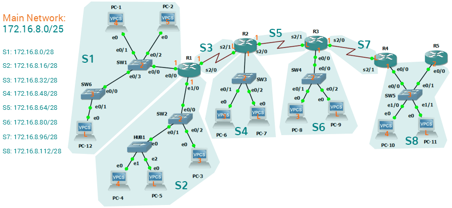
Tasks
- Configure the following hostnames to the appropriate switches:
- SW1 to Switch1
- SW2 to Switch2
- SW3 to Switch3
- SW4 to Switch4
- SW5 to Switch5
- SW6 to Switch6
- R1 to Router1
- R2 to Router2
- R3 to Router3
- R4 to Router4
- R5 to Router5
- Configure speed and duplex of 100-Full for all switches' and router's ethernet interfaces.
- Configure description on all interfaces with the format: Connected to <DeviceName> <PortNumber>. See samples below:
- In Switch1 e0/0: description is "Connected to Router1 e0/0".
- In Switch6 e0/1: description is "Connected to PC12 e0"
- Configure the enable password inclw on all switches and routers.
- Configure telnet password inclw on all switches and routers.
- Configure console password of inclw on all switches and routers.
- Verify using show commands if all configurations are applied.
- Save all switches and routers configurations.
Configurations
Subnet Design
INTERNOLD NETWORKS CCNA LIVE WEBCLASS (INCLW)
Subnet Design
Contents
Subnet Design
So far in this book, most of the discussion about IPv4 used examples with the addresses and masks already given. This book has shown many examples already, but the examples so far do not ask you to pick the IP address or pick the mask. Instead, as discussed back in Chapter 13, “Perspectives on IPv4 Subnetting,” this book so far has assumed that someone else designed the IP addressing and subnetting plan, and this book shows how to implement it.
This chapter turns that model around. It goes back to the progression of building and implementing IPv4, as discussed in Chapter 13, as shown in Figure 21-1. This chapter picks up the story right after some network engineer has chosen a Class A, B, or C network to use for the enterprise’s IPv4 network. And then this chapter discusses the design choices related to picking one subnet mask to use for all subnets (the first major section) and what subnet IDs that choice creates (the second major section).

Figure 21-1 Subnet Design and Implementation Process from Chapter 13
Note that Chapter 22, “Variable-Length Subnet Masks,” then changes the design choice of using a single mask, instead allowing any mask for each subnet through the use of variable-length subnet masks (VLSM).
Choosing the Mask(s) to Meet Requirements
This first major section examines how to find all the masks that meet the stated requirements for the number of subnets and the number of hosts per subnet. To that end, the text assumes that the designer has already determined these requirements and has chosen the network number to be subnetted. The designer has also made the choice to use a single subnet mask value throughout the classful network.
Armed with the information in this chapter, you can answer questions such as the following, a question that matters both for real engineering jobs and the Cisco exams:
You are using Class B network 172.16.0.0. You need 200 subnets and 200 hosts/subnet. Which of the following subnet mask(s) meet the requirements? (This question is then followed by several answers that list different subnet masks.)
To begin, this section reviews the concepts in Chapter 13’s section “Choose the Mask.” That section introduced the main concepts about how an engineer, when designing subnet conventions, must choose the mask based on the requirements.
After reviewing the related concepts from Chapter 13, this section examines this topic in more depth. In particular, this chapter looks at three general cases:
No masks meet the requirements.
One and only one mask meets the requirements.
Multiple masks meet the requirements.
For this last case, the text discusses how to determine all masks that meet the requirements and the trade-offs related to choosing which one mask to use.
Review: Choosing the Minimum Number of Subnet and Host Bits
The network designer must examine the requirements for the number of subnets and number of hosts/subnet, and then choose a mask. As discussed in detail in Chapter 15, “Analyzing Subnet Masks,” a classful view of IP addresses defines the three-part structure of an IP address: network, subnet, and host. The network designer must choose the mask so that the number of subnet and host bits (S and H, respectively, in Figure 21-2) meet the requirements.

Figure 21-2 Choosing the Number of Subnet and Host Bits
Basically, the designer must choose S subnet bits so that the number of subnets that can be uniquely numbered with S bits (2S) is at least as large as the required number of subnets. The designer applies similar logic to the number of host bits H, while noting that the formula is 2H – 2, because of the two reserved numbers in each subnet. So, keeping the powers of 2 handy, as shown in Table 21-2, will be useful when working through these problems.

Table 21-2 Powers of 2 Reference for Designing Masks
More formally, the process must determine the minimum values for both S and H that meet the requirements. The following list summarizes the initial steps to choose the mask:
Step 1. Determine the number of network bits (N) based on the class.
Step 2. Determine the smallest value of S, so that 2S => X, where X represents the required number of subnets.
Step 3. Determine the smallest value of H, so that 2H – 2 => Y, where Y represents the required number of hosts/subnet.
The next three sections examine how to use these initial steps to choose a subnet mask.
No Masks Meet Requirements
After you determine the required number of subnet and host bits, those bits might not fit into a 32-bit IPv4 subnet mask. Remember, the mask always has a total of 32 bits, with binary 1s in the network and subnet parts and binary 0s in the host part. For the exam, a question might provide a set of requirements that simply cannot be met with 32 total bits.
For example, consider the following sample exam question:
A network engineer is planning a subnet design. The engineer plans to use Class B network 172.16.0.0. The network has a need for 300 subnets and 280 hosts per subnet. Which of the following masks could the engineer choose?
The three-step process shown in the previous section shows that these requirements mean that a total of 34 bits will be needed, so no mask meets the requirements. First, as a Class B network, 16 network bits exist, with 16 host bits from which to create the subnet part and to leave enough host bits to number the hosts in each subnet. For the number of subnet bits, S=8 does not work, because 28 = 256 < 300. However, S=9 works, because 29 = 512 => 300. Similarly, because 28 – 2 = 254, which is less than 300, 8 host bits are not enough but 9 host bits (29 – 2 = 510) are just enough.
These requirements do not leave enough space to number all the hosts and subnet, because the network, subnet, and host parts add up to more than 32:
N=16, because as a Class B network, 16 network bits exist.
The minimum S=9, because S=8 provides too few subnets (28 = 256 < 300) but S=9 provides 29 = 512 subnets.
The minimum H=9, because H=8 provides too few hosts (28 – 2 = 254 < 280) but H=9 provides 29 – 2 = 510 hosts/subnet.
Figure 21-3 shows the resulting format for the IP addresses in this subnet, after the engineer has allocated 9 subnet bits on paper. Only 7 host bits remain, but the engineer needs 9 host bits.

Figure 21-3 Too Few Bits for the Host Part, Given the Requirements
One Mask Meets Requirements
The process discussed in this chapter in part focuses on finding the smallest number of subnet bits and the smallest number of host bits to meet the requirements. If the engineer tries to use these minimum values, and the combined network, subnet, and host parts add up to exactly 32 bits, exactly one mask meets the requirements.
For example, consider a revised version of the example in the previous section, with smaller numbers of subnet and hosts, as follows:
A network engineer is planning a subnet design. The engineer plans to use Class B network 172.16.0.0. The network has a need for 200 subnets and 180 hosts per subnet. Which of the following masks could the engineer choose?
The three-step process to determine the numbers of network, minimum subnet, and minimum host bits results in a need for 16, 8, and 8 bits, respectively. As before, with a Class B network, 16 network bits exist. With a need for only 200 subnets, S=8 does work, because 28 = 256 => 200; 7 subnet bits would not supply enough subnets (27 = 128). Similarly, because 28 – 2 = 254 => 180, 8 host bits meet the requirements; 7 host bits (for 126 total hosts/subnet) would not be enough.
Figure 21-4 shows the resulting format for the IP addresses in this subnet.

Figure 21-4 One Mask That Meets Requirements
Figure 21-4 shows the mask conceptually. To find the actual mask value, simply record the mask in prefix format (/P), where P = N + S or, in this case, /24.
Multiple Masks Meet Requirements
Depending on the requirements and choice of network, several masks might meet the requirements for the numbers of subnets and hosts/subnet. In these cases, you need to find all the masks that could be used. Then, you have a choice, but what should you consider when choosing one mask among all those that meet your requirements? This section shows how to find all the masks, as well as the facts to consider when choosing one mask from the list.
Finding All the Masks: Concepts
To help you better understand how to find all the subnet masks in binary, this section uses two major steps. In the first major step, you build the 32-bit binary subnet mask on paper. You write down binary 1s for the network bits, binary 1s for the subnet bits, and binary 0s for the host bits, just as always. However, you will use the minimum values for S and H. And when you write down these bits, you will not have 32 bits yet!
For example, consider the following problem, similar to the earlier examples in this chapter but with some changes in the requirements:
A network engineer is planning a subnet design. The engineer plans to use Class B network 172.16.0.0. The network has a need for 50 subnets and 180 hosts per subnet. Which of the following masks could the engineer choose?
This example is similar to an earlier example, except that only 50 subnets are needed in this case. Again, the engineer is using private IP network 172.16.0.0, meaning 16 network bits. The design requires only 6 subnet bits in this case, because 26 = 64 => 50, and with only 5 subnet bits, 25 = 32 < 50. The design then requires a minimum of 8 host bits.
One way to discuss the concepts and find all the masks that meet these requirements is to write down the bits in the subnet mask: binary 1s for the network and subnet parts and binary 0s for the host part. However, think of the 32-bit mask as 32-bit positions, and when writing the binary 0s, write them on the far right. Figure 21-5 shows the general idea.

Figure 21-5 Incomplete Mask with N=16, S=6, and H=8
Figure 21-5 shows 30 bits of the mask, but the mask must have 32 bits. The 2 remaining bits might become subnet bits, being set to binary 1. Alternatively, these 2 bits could be made host bits, being set to binary 0. The engineer simply needs to choose based on whether he would like more subnet bits, to number more subnets, or more host bits, to number more hosts/subnet.
Regardless of the requirements, when choosing any IPv4 subnet mask, you must always follow this rule:
A subnet mask begins with all binary 1s, followed by all binary 0s, with no interleaving of 1s and 0s.
With the example shown in Figure 21-5, with 2 open bits, one value (binary 01) breaks this rule. However, the other three combinations of 2 bits (00, 10, and 11) do not break the rule. As a result, three masks meet the requirements in this example, as shown in Figure 21-6.

Figure 21-6 Three Masks That Meet the Requirements
In the three masks, the first has the least number of subnet bits among the three masks, but therefore has the most number of host bits. So, the first mask maximizes the number of hosts/subnet. The last mask uses the minimum value for the number of host bits, therefore using the most number of subnet bits allowed while still meeting the requirements. As a result, the last mask maximizes the number of subnets allowed.
Finding All the Masks: Math
Although the concepts related to the example shown in Figures 21-5 and 21-6 are important, you can find the range of masks that meets the requirements more easily just using some simple math. The process to find the masks just requires a few steps, after you know N and the minimum values of S and H. The process finds the value of /P when using the least number of subnet bits, and when using the least number of host bits, as follows:
Step 1. Calculate the shortest prefix mask (/P) based on the minimum value of S, where P = N + S.
Step 2. Calculate the longest prefix mask (/P) based on the minimum value of H, where P = 32 – H.
Step 3. The range of valid masks includes all /P values between the two values calculated in the previous steps.
For example, in the example shown in Figure 21-6, N = 16, the minimum S = 6, and the minimum H = 8. The first step identifies the shortest prefix mask (the /P with the smallest value of P) of /22 by adding N and S (16 + 6). The second step identifies the longest prefix mask that meets the requirements by subtracting the smallest possible value for H (8, in this case) from 32, for a mask of /24. The third step reminds us that the range is from /22 to /24, meaning that /23 is also an option.
Choosing the Best Mask
When multiple possible masks meet the stated requirements, the engineer has a choice of masks. That, of course, begs some questions: Which mask should you choose? Why would one mask be better than the other? The reasons can be summarized into three main options:
To maximize the number of hosts/subnet: To make this choice, use the shortest prefix mask (that is, the mask with the smallest /P value), because this mask has the largest host part.
To maximize the number of subnets: To make this choice, use the longest prefix mask (that is, the mask with the largest /P value), because this mask has the largest subnet part.
To increase both the numbers of supported subnets and hosts: To make this choice, choose a mask in the middle of the range, which gives you both more subnet bits and more host bits.
For example, in Figure 21-6, the range of masks that meet the requirements is /22 – /24. The shortest mask, /22, has the least subnet bits but the largest number of host bits (10) of the three answers, maximizing the number of hosts/subnet. The longest mask, /24, maximizes the number of subnet bits (8), maximizing the number of subnets, at least among the options that meet the original requirements. The mask in the middle, /23, provides some growth in both subnets and hosts/subnet.
The Formal Process
Although this chapter has explained various steps in finding a subnet mask to meet the design requirements, it has not yet collected these concepts into a list for the entire process. The following list collects all these steps into one place for reference. Note that this list does not introduce any new concepts compared to the rest of this chapter; it just puts all the ideas in one place.
Step 1. Find the number of network bits (N) per class rules.
Step 2. Calculate the minimum number of subnet bits (S) so that 2S => the number of required subnets.
Step 3. Calculate the minimum number of host bits (H) so that 2H – 2 => the number of required hosts/subnet.
Step 4. If N + S + H > 32, no mask meets the need.
Step 5. If N + S + H = 32, one mask meets the need. Calculate the mask as /P, where P = N + S.
Step 6. If N + S + H < 32, multiple masks meet the need:
A. Calculate mask /P based on the minimum value of S, where P = N + S. This mask maximizes the number of hosts/subnet.
B. Calculate mask /P based on the minimum value of H, where P = 32 – H. This mask maximizes the number of possible subnets.
C. Note that the complete range of masks includes all prefix lengths between the two values calculated in Steps 6A and 6B.
Practice Choosing Subnet Masks
Take the usual two-phase approach to learning new subnetting math and processes. Take the time now to practice to make sure you understand the fundamentals, using the book and notes as needed. Then, sometime before taking the exam, practice until you can reach the goals in the right column of Table 21-3.

Table 21-3 Keep-Reading and Take-Exam Goals for Choosing a Subnet Mask
Practice Problems for Choosing a Subnet Mask
The following list shows three separate problems, each with a classful network number and a required number of subnets and hosts/subnet. For each problem, determine the minimum number of subnet and host bits that meet the requirements. If more than one mask exists, note which mask maximizes the number of hosts/subnet and which maximizes the number of subnets. If only one mask meets the requirements, simply list that mask. List the masks in prefix format:
1. Network 10.0.0.0, need 1500 subnets, need 300 hosts/subnet
2. Network 172.25.0.0, need 130 subnets, need 127 hosts/subnet
3. Network 192.168.83.0, need 8 subnets, need 8 hosts/subnet
Table 21-8, found in the later section “Answers to Earlier Practice Problems,” lists the answers.
Finding All Subnet IDs
After the person designing the IP subnetting plan has chosen the one mask to use throughout the Class A, B, or C network, he will soon need to start assigning specific subnet IDs for use in specific VLANs, serial links, and other places in the internetwork that need a subnet. But what are those subnet IDs? As it turns out, after the network ID and one subnet mask for all subnets have been chosen, finding all the subnet IDs just requires doing a little math. This second major section of this chapter focuses on that math, which focuses on a single question:
Given a single Class A, B, or C network, and the single subnet mask to use for all subnets, what are all the subnet IDs?
When learning how to answer this question, you can think about the problem in either binary or decimal. This chapter approaches the problem using decimal. Although the process itself requires only simple math, the process requires practice before most people can confidently answer this question.
The decimal process begins by identifying the first, or numerically lowest, subnet ID. After that, the process identifies a pattern in all subnet IDs for a given subnet mask so that you can find each successive subnet ID through simple addition. This section examines the key ideas behind this process first; then you are given a formal definition of the process.
NOTE: Some videos included on the accompanying DVD describe the same fundamental processes to find all subnet IDs. You can view those videos before or after reading this section, or even instead of reading this section, as long as you learn how to independently find all subnet IDs. The process step numbering in the videos might not match the steps shown in this edition of the book.
First Subnet ID: The Zero Subnet
The first step in finding all subnet IDs of one network is incredibly simple: Copy the network ID. That is, take the Class A, B, or C network ID—in other words, the classful network ID—and write it down as the first subnet ID. No matter what Class A, B, or C network you use, and no matter what subnet mask you use, the first (numerically lowest) subnet ID is equal to the network ID.
For example, if you begin with classful network 172.20.0.0, no matter what the mask is, the first subnet ID is 172.20.0.0.
This first subnet ID in each network goes by two special names: either subnet zero or the zero subnet. The origin of these names is related to the fact that a network’s zero subnet, when viewed in binary, has a subnet part of all binary 0s. In decimal, the zero subnet can be easily identified, because the zero subnet always has the exact same numeric value as the network ID itself.
In the past, engineers avoided using zero subnets because of the ambiguity with one number that could represent the entire classful network or it could represent one subnet inside the classful network. To help control that, IOS has a global command that can be set one of two ways:
ip subnet-zero, which allows the configuration of addresses in the zero subnet.
no ip subnet-zero, which prevents the configuration of addresses in the zero subnet.
Although most sites use the default setting to allow zero subnets, you can use the no ip subnet-zero command to prevent configuring addresses that are part of a zero subnet. Example 21-1 shows how a router rejects an ip address command after changing to use no ip subnet-zero. Note that the error message does not mention the zero subnet, instead simply stating “bad mask.”
Example 21-1 Effects of [no] ip subnet-zero on a Local Router

Note that the no ip subnet-zero command affects the local router’s ip address commands, as well as the local router’s ip route commands (which define static routes). However, it does not affect the local router’s routes as learned with a routing protocol.
Finding the Pattern Using the Magic Number
Subnet IDs follow a predictable pattern, at least when using our assumption of a single subnet mask for all subnets of a network. The pattern uses the magic number, as discussed in Chapter 16, “Analyzing Existing Subnets.” To review, the magic number is 256, minus the mask’s decimal value, in a particular octet that this book refers to as the interesting octet.
Figure 21-7 shows four examples of these patterns with four different masks. For example, just look at the top of the figure to start. It lists mask 255.255.128.0 on the left. The third octet is the interesting octet, with a mask value other than 0 or 255 in that octet. The left side shows a magic number calculated as 256 – 128 = 128. So, the pattern of subnet IDs is shown in the highlighted number line; that is, the subnet IDs when using this mask will have either a 0 or 128 in the third octet. For example, if using network 172.16.0.0, the subnet IDs would be 172.16.0.0 and 172.16.128.0.

Figure 21-7 Patterns with Magic Numbers for Masks /17 – /20
Now focus on the second row, with another example, with mask 255.255.192.0. This row shows a magic number of 64 (256 – 192 = 64), so the subnet IDs will use a value of 0, 64, 128, or 192 (multiples of 64) in the third octet. For example, if used with network 172.16.0.0, the subnet IDs would be 172.16.0.0, 172.16.64.0, 172.16.128.0, and 172.16.192.0.
Looking at the third row/example, the mask is 255.255.224.0, with a magic number of 256 – 224 = 32. So, as shown in the center of the figure, the subnet ID values will be multiples of 32. For example, if used with network 172.16.0.0 again, this mask would tell us that the subnet IDs are 172.16.0.0, 172.16.32.0, 172.16.64.0, 172.16.96.0, and so on.
Finally, for the bottom example, mask 255.255.240.0 makes the magic number, in the third octet, be 16. So, all the subnet IDs will be a multiple of 16 in the third octet, with those values shown in the middle of the figure.
A Formal Process with Less Than 8 Subnet Bits
Although it can be easy to see the patterns in Figure 21-7, it might not be as obvious exactly how to apply those concepts to find all the subnet IDs in every case. This section outlines a specific process to find all the subnet IDs.
To simplify the explanations, this section assumes that less than 8 subnet bits exist. Later, the section “Finding All Subnets with More Than 8 Subnet Bits,” describes the full process that can be used in all cases.
First, to organize your thoughts, you might want to organize the data into a table like Table 21-4. This book refers to this chart as the list-all-subnets chart.

Table 21-4 Generic List-All-Subnets Chart
A formal process to find all subnet IDs, given a network and a single subnet mask, is as follows:
Step 1. Write down the subnet mask, in decimal, in the first empty row of the table.
Step 2. Identify the interesting octet, which is the one octet of the mask with a value other than 255 or 0. Draw a rectangle around the column of the interesting octet.
Step 3. Calculate and write down the magic number by subtracting the subnet mask’s interesting octet from 256.
Step 4. Write down the classful network number, which is the same number as the zero subnet, in the next empty row of the list-all-subnets chart.
Step 5. To find each successive subnet number:
A. For the three uninteresting octets, copy the previous subnet number’s values.
B. For the interesting octet, add the magic number to the previous subnet number’s interesting octet.
Step 6. When the sum calculated in Step 5B reaches 256, stop the process. The number with the 256 in it is out of range, and the previous subnet number is the broadcast subnet.
Although the written process is long, with practice, most people can find the answers much more quickly with this decimal-based process than by using binary math. As usual, most people learn this process best by seeing it in action, exercising it, and then practicing it. To that end, review the two following examples and watch any videos that came with this book that show additional examples.
Example 1: Network 172.16.0.0, Mask 255.255.240.0
To begin this example, focus on the first four of the six steps, when subnetting network 172.16.0.0 using mask 255.255.240.0. Figure 21-8 shows the results of these first four steps:
Step 1. Record mask 255.255.240.0, which was given as part of the problem statement. (Figure 21-8 also shows the network ID, 172.16.0.0, for easy reference.)
Step 2. The mask’s third octet is neither 0 nor 255, which makes the third octet interesting.
Step 3. Because the mask’s value in the third octet is 240, the magic number = 256 – 240 = 16.
Step 4. Because the network ID is 172.16.0.0, the first subnet ID, the zero subnet, is also 172.16.0.0.

Figure 21-8 Results of First Four Steps: 172.16.0.0, 255.255.240.0.
These first four steps discover the first subnet (the zero subnet) and get you ready to do the remaining steps by identifying the interesting octet and the magic number. Step 5 in the process tells you to copy the three boring octets and add the magic number (16, in this case) in the interesting octet (octet 3, in this case). Keep repeating this step until the interesting octet value equals 256 (per Step 6). When the total is 256, you have listed all the subnet IDs, and the line with 256 on it is not a correct subnet ID. Figure 21-9 shows the results of the Step 5 actions.

Figure 21-9 List of Subnet IDs: 172.16.0.0, 255.255.240.0
NOTE: In any list of all the subnet IDs of a network, the numerically highest subnet ID is called the broadcast subnet. Decades ago, engineers avoided using the broadcast subnet. However, using the broadcast subnet causes no problems. The term broadcast subnet has its origins in the fact that if you determine the subnet broadcast address inside the broadcast subnet, it has the same numeric value as the network-wide broadcast address.
NOTE: People sometimes confuse the terms broadcast subnet and subnet broadcast address. The broadcast subnet is one subnet, namely the numerically highest subnet; only one such subnet exists per network. The term subnet broadcast address refers to the one number in each and every subnet that is the numerically highest number in that subnet.
Example 2: Network 192.168.1.0, Mask 255.255.255.224
With a Class C network and a mask of 255.255.255.224, this example makes the fourth octet the interesting octet. However, the process works the same, with the same logic, just with the interesting logic applied in a different octet. As with the previous example, the following list outlines the first four steps, with Figure 21-10 showing the results of the first four steps:
Step 1. Record mask 255.255.255.224, which was given as part of the problem statement, and optionally record the network number (192.168.1.0).
Step 2. The mask’s fourth octet is neither 0 nor 255, which makes the fourth octet interesting.
Step 3. Because the mask’s value in the fourth octet is 224, the magic number = 256 – 224 = 32.
Step 4. Because the network ID is 192.168.1.0, the first subnet ID, the zero subnet, is also 192.168.1.0.

Figure 21-10 Results of First Four Steps: 192.168.1.0, 255.255.255.224
From this point, Step 5 in the process tells you to copy the values in the first three octets and then add the magic number (32, in this case) in the interesting octet (octet 4, in this case). Keep doing so until the interesting octet value equals 256 (per Step 6). When the total is 256, you have listed all the subnet IDs, and the line with 256 on it is not a correct subnet ID. Figure 21-11 shows the results of these steps.

Figure 21-11 List of Subnet IDs: 192.168.1.0, 255.255.255.224
Finding All Subnets with Exactly 8 Subnet Bits
The formal process in the earlier section “A Formal Process with Less Than 8 Subnet Bits” identified the interesting octet as the octet whose mask value is neither a 255 nor a 0. If the mask defines exactly 8 subnet bits, you must use a different logic to identify the interesting octet; otherwise, the same process can be used. In fact, the actual subnet IDs can be a little more intuitive.
Only two cases exist with exactly 8 subnet bits:
A Class A network with mask 255.255.0.0; the entire second octet contains subnet bits.
A Class B network with mask 255.255.255.0; the entire third octet contains subnet bits.
In each case, use the same process as with less than 8 subnet bits, but identify the interesting octet as the one octet that contains subnet bits. Also, because the mask’s value is 255, the magic number will be 256 – 255 = 1, so the subnet IDs are each 1 larger than the previous subnet ID.
For example, for 172.16.0.0, mask 255.255.255.0, the third octet is the interesting octet and the magic number is 256 – 255 = 1. You start with the zero subnet, equal in value to network number 172.16.0.0, and then add 1 in the third octet. For example, the first four subnets are as follows:
172.16.0.0 (zero subnet)
172.16.1.0
172.16.2.0
172.16.3.0
Finding All Subnets with More Than 8 Subnet Bits
Earlier, the section “A Formal Process with Less Than 8 Subnet Bits” assumed less than 8 subnet bits for the purpose of simplifying the discussions while you learn. In real life, you need to be able to find all subnet IDs with any valid mask, so you cannot assume less than 8 subnet bits.
The examples that have at least 9 subnet bits have a minimum of 512 subnet IDs, so writing down such a list would take a lot of time. To conserve space, the examples will use shorthand rather than list hundreds or thousands of subnet IDs.
The process with less than 8 subnet bits told you to count in increments of the magic number in one octet. With more than 8 subnet bits, the new expanded process must tell you how to count in multiple octets. So, this section breaks down two general cases: (a) when 9–16 subnet bits exist, which means that the subnet field exists in only two octets, and (b) cases with 17 or more subnet bits, which means that the subnet field exists in three octets.
Process with 9–16 Subnet Bits
To understand the process, you need to know a few terms that the process will use. Figure 21-12 shows the details, with an example that uses Class B network 130.4.0.0 and mask 255.255.255.192. The lower part of the figure details the structure of the addresses per the mask: a network part of two octets because it is a Class B address, a 10-bit subnet part per the mask (/26), and 6 host bits.

Figure 21-12 Fundamental Concepts and Terms for the >8 Subnet Bit Process
In this case, subnet bits exist in two octets: octets 3 and 4. For the purposes of the process, the rightmost of these octets is the interesting octet, and the octet just to the left is the cleverly named just-left octet.
The updated process, which makes adjustments for cases in which the subnet field is longer than 1 octet, tells you to count in increments of the magic number in the interesting octet, but count by 1s in the just-left octet. Formally:
Step 1. Calculate subnet IDs using the 8-subnet-bits-or-less process. However, when the total adds up to 256, move to the next step; consider the subnet IDs listed so far as a subnet block.
Step 2. Copy the previous subnet block, but add 1 to the just-left octet in all subnet IDs in the new block.
Step 3. Repeat Step 2 until you create the block with a just-left octet of 255, but go no further.
To be honest, the formal concept can cause you problems until you work through some examples, so even if the process remains a bit unclear in your mind, you should work through the following examples instead of rereading the formal process.
First, consider an example based on Figure 21-12, with network 130.4.0.0 and mask 255.255.255.192. Figure 21-12 already showed the structure, and Figure 21-13 shows the subnet ID block created at Step 1.

Figure 21-13 Step 1: Listing the First Subnet ID Block
The logic at Step 1, to create this subnet ID block of four subnet IDs, follows the same magic number process seen before. The first subnet ID, 130.4.0.0, is the zero subnet. The next three subnet IDs are each 64 bigger, because the magic number, in this case, is 256 – 192 = 64.
Steps 2 and 3 from the formal process tell you how to create 256 subnet blocks, and by doing so, you will list all 1024 subnet IDs. To do so, create 256 total subnet blocks: one with a 0 in the just-left octet, one with a 1 in the just-left octet, and another with a 2 in the just-left octet, up through 255. The process continues through the step at which you create the subnet block with 255 in the just-left octet (third octet, in this case). Figure 21-14 shows the idea, with the addition of the first few subnet blocks.

Figure 21-14 Step 2: Replicating the Subnet Block with +1 in the Just-Left Octet
This example, with 10 total subnet bits, creates 256 blocks of four subnets each, for a total of 1024 subnets. This math matches the usual method of counting subnets, because 210 = 1024.
Process with 17 or More Subnet Bits
To create a subnet design that allows 17 or more subnet bits to exist, the design must use a Class A network. In addition, the subnet part will consist of the entire second and third octets, plus part of the fourth octet. That means a lot of subnet IDs: at least 217 (or 131,072) subnets. Figure 21-15 shows an example of just such a structure, with a Class A network and a /26 mask.

Figure 21-15 Address Structure with 18 Subnet Bits
To find all the subnet IDs in this example, you use the same general process as with 9–16 subnet bits, but with many more subnet blocks to create. In effect, you have to create a subnet block for all combinations of values (0–255, inclusive) in both the second and third octet. Figure 21-16 shows the general idea. Note that with only 2 subnet bits in the fourth octet in this example, the subnet blocks will have four subnets each.

Figure 21-16 256 Times 256 Subnet Blocks of Four Subnets
Practice Finding All Subnet IDs
Before moving to the next chapter, practice until you get the right answer most of the time—but use any tools you want and take all the time you need. Then, you can move on with your reading. Before taking the exam, practice until you reach the goals in the right column of Table 21-5, which summarizes the key concepts and suggestions for this two-phase approach.

Table 21-5 Keep-Reading and Take-Exam Goals for This Chapter’s Topics
Practice Problems for Finding All Subnet IDs
The following list shows three separate problems, each with a classful network number and prefix-style mask. Find all subnet IDs for each problem:
1. 192.168.9.0/27
2. 172.30.0.0/20
3. 10.0.0.0/17
The section “Answers to Earlier Practice Problems,” later in this chapter, lists the answers.
