

Analyzing Ethernet LAN Switching
INTERNOLD NETWORKS CCNA LIVE WEBCLASS (INCLW)
Analyzing Ethernet LAN Switching
Contents
Analyzing Ethernet LAN Switching
When you buy a Cisco Catalyst Ethernet switch, the switch is ready to work.
All you have to do is take it out of the box, power on the switch by connecting the power cable to the switch and a power outlet, and connect hosts to the switch using the correct unshielded twisted-pair (UTP) cables.
You do not have to configure anything else, you do not have to connect to the console and login, or do anything: the switch just starts forwarding Ethernet frames.
In later lessons, you will learn how to build, configure, and verify the operation of Ethernet LANs.
In the lesson, “Using the Command-Line Interface,” you learned some skills so you know how to connect to a switch’s CLI, move around in the CLI, issue commands, and configure the switch.
The next step—this lesson—takes a short but important step in that journey by explaining the logic a switch uses when forwarding Ethernet frames.
This lesson has two major sections. The first reviews the concepts behind LAN switching, which were first introduced back in previous lesson, “Fundamentals of Ethernet LANs.”
The second section of this lesson then uses IOS show commands to verify that Cisco switches actually learned the MAC addresses, built its MAC address table, and forwarded frames.
LAN Switching Concepts
A modern Ethernet LAN connects user devices as well as servers into some switches, with the switches then connecting to each other, sometimes in a design like Figure 1.
Part of the LAN, called a campus LAN, supports the end user population as shown on the left of the figure. End user devices connect to LAN switches, which in turn connect to other switches so that a path exists to the rest of the network.
The campus LAN switches sit in wiring closets close to the end users. On the right, the servers used to provide information to the users also connects to the LAN.
Those servers and switches often sit in a closed room called a data center, with connections to the campus LAN to support traffic to/from the users.

Figure 1: Campus LAN and Data Center LAN, Conceptual Drawing
To forward traffic from a user device to a server and back, each switch performs the same kind of logic, independently from each other.
The first half of this lesson examines the logic: how a switch chooses to forward an Ethernet frame, when the switch chooses to not forward the frame, and so on.
Overview of Switching Logic
Ultimately, the role of a LAN switch is to forward Ethernet frames.
LANs exist as a set of user devices, servers, and other devices that connect to switches, with the switches connected to each other. The LAN switch has one primary job: to forward frames to the correct destination (MAC) address.
And to achieve that goal, switches use logic—logic based on the source and destination MAC address in each frame’s Ethernet header.
LAN switches receive Ethernet frames and then make a switching decision: either forward the frame out some other ports or ignore the frame. To accomplish this primary mission, switches perform three actions:
- Deciding when to forward a frame or when to filter (not forward) a frame, based on the destination MAC address.
- Preparing to forward frames by learning MAC addresses by examining the source MAC address of each frame received by the switch.
- Preparing to forward only one copy of the frame to the destination by creating a (Layer 2) loop-free environment with other switches by using Spanning Tree Protocol (STP).
The first action is the switch’s primary job, whereas the other two items are overhead functions.
NOTE: Throughout our discussion of LAN switches, the terms switch port and switch interface are synonymous.
Although previous lessons already discussed the frame format, this discussion of Ethernet switching is pretty important, so reviewing the Ethernet frame at this point might be helpful.
Figure 2 shows one popular format for an Ethernet frame.
Basically, a switch would take the frame shown in the figure, make a decision of where to forward the frame, and send the frame out that other interface.

Figure 2: IEEE 802.3 Ethernet Frame (One Variation)
Most of the upcoming discussions and figures about Ethernet switching focuses on the use of the destination and source MAC address fields in the header.
All Ethernet frames have both a destination and source MAC address.
Both are 6-bytes long (represented as 12 hex digits), and are a key part of the switching logic discussed in this section.
Forwarding Known Unicast Frames
To decide whether to forward a frame, a switch uses a dynamically built table that lists MAC addresses and outgoing interfaces. Switches compare the frame’s destination MAC address to this table to decide whether the switch should forward a frame or simply ignore it.
For example, consider the simple network shown in Figure 3, with Fred sending a frame to Barney.

Figure 3: Sample Switch Forwarding and Filtering Decision
In this figure, Fred sends a frame with destination address 0200.2222.2222 (Barney’s MAC address).
The switch compares the destination MAC address (0200.2222.2222) to the MAC address table, matching the bold table entry.
That matched table entry tells the switch to forward the frame out port F0/2, and only port F0/2.
NOTE: A switch’s MAC address table is also called the switching table, or bridging table, or even the Content-Addressable Memory (CAM) table, in reference to the type of physical memory used to store the table.
A switch’s MAC address table lists the location of each MAC relative to that one switch. In LANs with multiple switches, each switch makes an independent forwarding decision based on its own MAC address table. Together, they forward the frame so that it eventually arrives at the destination.
For example, Figure 4 shows the first switching decision in a case in which Fred sends a frame to Wilma, with destination MAC 0200.3333.3333.
The topology has changed versus the previous figure, this time with two switches, and Fred and Wilma connected to two different switches.
Figure 3 shows the first switch’s logic, in reaction to Fred sending the original frame. Basically, the switch receives the frame in port F0/1, finds the destination MAC (0200.3333.3333) in the MAC address table, sees the outgoing port of G0/1, so SW1 forwards the frame out its G0/1 port.

Figure 4: Forwarding Decision with Two Switches: First Switch
That same frame next arrives at switch SW2, entering SW2’s G0/2 interface.
As shown in Figure 5, SW2 uses the same logic steps, but using SW2’s table. The MAC table lists the forwarding instructions for that switch only. In this case, switch SW2 forwards the frame out its F0/3 port, based on SW2’s MAC address table.

Figure 5: Forwarding Decision with Two Switches: Second Switch
NOTE: The forwarding choice by a switch was formerly called a forward-versus-filter decision, because the switch also chooses to not forward (to filter) frames, not sending the frame out some ports.
The examples so far use switches that happen to have a MAC table with all the MAC addresses listed.
As a result, the destination MAC address in the frame is known to the switch. The frames are called known unicast frames, or simply known unicasts, because the destination address is a unicast address, and the destination is known.
As shown in these examples, switches forward known unicast frames out one port: the port as listed in the MAC table entry for that MAC address.
Learning MAC Addresses
Thankfully, the networking staff does not have to type in all those MAC table entries. Instead, the switches do their second main function: to learn the MAC addresses and interfaces to put into its address table.
With a complete MAC address table, the switch can make accurate forwarding and filtering decisions as just discussed.
Switches build the address table by listening to incoming frames and examining the source MAC address in the frame. If a frame enters the switch and the source MAC address is not in the MAC address table, the switch creates an entry in the table. That table entry lists the interface from which the frame arrived. Switch learning logic is that simple.
Figure 6 depicts the same single-switch topology network as Figure 3, but before the switch has built any address table entries.
The figure shows the first two frames sent in this network—first a frame from Fred, addressed to Barney, and then Barney’s response, addressed to Fred.

Figure 6: Switch Learning: Empty Table and Adding Two Entries
(Figure 6 depicts the MAC learning process only, and ignores the forwarding process and therefore ignores the destination MAC addresses.)
Focus on the learning process and how the MAC table grows at each step as shown on the right side of the figure.
The switch begins with an empty MAC table, as shown in the upper right part of the figure. Then Fred sends his first frame (labeled “1”) to Barney, so the switch adds an entry for 0200.1111.1111, Fred’s MAC address, associated with interface F0/1.
Why F0/1? The frame sent by Fred entered the switch’s F0/1 port. SW1’s logic runs something like this: “The source is MAC 0200.1111.1111, the frame entered F0/1, so from my perspective, 0200.1111.1111 must be reachable out my port F0/1.”
Continuing the example, when Barney replies in Step 2, the switch adds a second entry, this one for 0200.2222.2222, Barney’s MAC address, along with interface F0/2. Why F0/2? The frame Barney sent entered the switch’s F0/2 interface. Learning always occurs by looking at the source MAC address in the frame, and adds the incoming interface as the associated port.
Flooding Unknown Unicast and Broadcast Frames
Now again turn your attention to the forwarding process, using the topology in Figure 5. What do you suppose the switch does with Fred’s first frame, the one that occurred when there were no entries in the MAC address table?
As it turns out, when there is no matching entry in the table, switches forward the frame out all interfaces (except the incoming interface) using a process called flooding. And the frame whose destination address is unknown to the switch is called an unknown unicast frame, or simply an unknown unicast.
Switches flood unknown unicast frames. Flooding means that the switch forwards copies of the frame out all ports, except the port on which the frame was received.
The idea is simple: if you do not know where to send it, send it everywhere, to deliver the frame. And, by the way, that device will likely then send a reply—and then the switch can learn that device’s MAC address, and forward future frames out one port as a known unicast frame.
Switches also flood LAN broadcast frames (frames destined to the Ethernet broadcast address of FFFF.FFFF.FFFF), because this process helps deliver a copy of the frame to all devices in the LAN.
For example, Figure 7 shows the same first frame sent by Fred, when the switch’s MAC table is empty. At step 1, Fred sends the frame. At step 2, the switch sends a copy of the frame out all three of the other interfaces.

Figure 7: Switch Flooding: Unknown Unicast Arrives, Floods out Other Ports
Avoiding Loops Using Spanning Tree Protocol
The third primary feature of LAN switches is loop prevention, as implemented by Spanning Tree Protocol (STP). Without STP, any flooded frames would loop for an indefinite period of time in Ethernet networks with physically redundant links.
To prevent looping frames, STP blocks some ports from forwarding frames so that only one active path exists between any pair of LAN segments.
The result of STP is good: Frames do not loop infinitely, which makes the LAN usable. However, STP has negative features as well, including the fact that it takes some work to balance traffic across the redundant alternate links.
A simple example makes the need for STP more obvious. Remember, switches flood unknown unicast frames and broadcast frames.
Figure 8 shows an unknown unicast frame, sent by Larry to Bob, which loops forever because the network has redundancy but no STP. Note that the figure shows one direction of the looping frame only, just to reduce clutter, but a copy of the frame would also loop the other direction as well.

Figure 8: Network with Redundant Links but Without STP: The Frame Loops Forever
The flooding of this frame would cause the frame to rotate around the three switches, because none of the switches list Bob’s MAC address in their address tables, each switch floods the frame.
And while the flooding process is a good mechanism for forwarding unknown unicasts and broadcasts, the continual flooding of traffic frames as in the figure can completely congest the LAN to the point of making it unusable.
A topology like Figure 8, with redundant links, is good, but we need to prevent the bad effect of those looping frames. To avoid Layer 2 loops, all switches need to use STP. STP causes each interface on a switch to settle into either a blocking state or a forwarding state.
Blocking means that the interface cannot forward or receive data frames, while forwarding means that the interface can send and receive data frames. If a correct subset of the interfaces is blocked, only a single currently active logical path exists between each pair of LANs.
NOTE: STP behaves identically for a transparent bridge and a switch. Therefore, the terms bridge, switch, and bridging device all are used interchangeably when discussing STP.
LAN Switching Summary
Switches use Layer 2 logic, examining the Ethernet data-link header to choose how to process frames. In particular, switches make decisions to forward and filter frames, learn MAC addresses, and use STP to avoid loops, as follows:
- Step 1. Switches forward frames based on the destination MAC address:
- A. If the destination MAC address is a broadcast, multicast, or unknown destination unicast (a unicast not listed in the MAC table), the switch floods the frame.
- B. If the destination MAC address is a known unicast address (a unicast address found in the MAC table):
- i. If the outgoing interface listed in the MAC address table is different from the interface in which the frame was received, the switch forwards the frame out the outgoing interface.
- ii. If the outgoing interface is the same as the interface in which the frame was received, the switch filters the frame, meaning that the switch simply ignores the frame and does not forward it.
- Step 2. Switches use the following logic to learn MAC address table entries:
- A. For each received frame, examine the source MAC address and note the interface from which the frame was received.
- B. If it is not already in the table, add the MAC address and interface it was learned on.
- Step 3. Switches use STP to prevent loops by causing some interfaces to block, meaning that they do not send or receive frames.
Verifying and Analyzing Ethernet Switching
A Cisco Catalyst switch comes from the factory ready to switch frames. All you have to do is connect the power cable, plug in the Ethernet cables, and the switch starts switching incoming frames.
Connect multiple switches together, and they are ready to forward frames between the switches as well. And the big reason behind this default behavior has to do with the default settings on the switches.
Cisco Catalyst switches come ready to get busy switching frames because of settings like these:
- The interfaces are enabled by default, ready to start working once a cable is connected.
- All interfaces are assigned to VLAN 1.
- 10/100 and 10/100/1000 interfaces use autonegotiation by default.
- The MAC learning, forwarding, flooding logic all works by default.
- STP is enabled by default.
This second section of the lesson examines how switches will work with these default settings, showing how to verify the Ethernet learning and forwarding process.
Demonstrating MAC Learning
To see a switches MAC address table, use the show mac address-table command.
With no additional parameters, this command lists all known MAC addresses in the MAC table, including some overhead static MAC addresses that you can ignore.
To see all the dynamically learned MAC addresses only, instead use the show mac address-table dynamic command.
The examples in this lesson use almost no configuration, as if you just unboxed the switch when you first purchased it.
For the examples, the switches have no configuration other than the hostname command to set a meaningful hostname.
Note that to do this in lab:
- Image Use the erase startup-config EXEC command to erase the startup-config file
- Image Use the delete vlan.dat EXEC command to delete the VLAN configuration details
- Image Use the reload EXEC command to reload the switch (thereby using the empty startup-config, with no VLAN information configured)
- Image Configure the hostname SW1 command to set the switch hostname
Once done, the switch starts forwarding and learning MAC address, as demonstrated in Example 1.

Example 1: show mac address-table dynamic
First, focus on two columns of the table: the Mac Address and Ports columns of the table. The values should look familiar: they match the earlier single-switch example, as repeated here as Figure 9.
Note the four MAC addresses listed, along with their matching ports, as shown in the figure.

Figure 9: Single Switch Topology Used in Verification Section
Next, look at the Type field in the header. The column tells us whether the MAC address was learned by the switch as described earlier in this lesson.
You can also statically predefine MAC table entries using a couple of different features, including port security, and those would appear as Static in the Type column.
Finally, the VLAN column of the output gives us a chance to briefly discuss how VLANs impact switching logic. LAN switches forward Ethernet frames inside a VLAN.
What that means is if a frame enters via a port in VLAN 1, then the switch will forward or flood that frame out other ports in VLAN 1 only, and not out any ports that happen to be assigned to another VLAN.
Details of VLANs will be discuss in other lessons.
Switch Interfaces
The first example assumes that you installed the switch and cabling correctly, and that the switch interfaces work. Once you do the installation and connect to the Console, you can easily check the status of those interfaces with the show interfaces status command, as shown in Example 2.


Example 2: show interfaces status on Switch SW1
Focus on the port column for a moment.
As a reminder, Cisco Catalyst switches name their ports based on the fastest specification supported, so in this case, the switch has 24 interfaces named Fast Ethernet, and two named Gigabit Ethernet.
Many commands abbreviate those terms, this time as Fa for Fast Ethernet and Gi for Gigabit Ethernet. (The example happens to come from a Cisco Catalyst switch that has 24 10/100 ports and two 10/100/1000 ports.)
The Status column of course tells us the status or state of the port. In this case, the lab switch had cables and devices connected to ports F0/1–F0/4 only, with no other cables connected. As a result, those first four ports have a state of connected, meaning that the ports have a cable and are functional.
The notconnect state means that the port is not yet functioning. It may mean that there is no cable installed, but other problems may exist as well.
NOTE: You can see the status for a single interface in a couple of ways. For instance, for F0/1, the command show interfaces f0/1 status lists the status in a single line of output as in Example 2. The show interfaces f0/1 command (without the status keyword) displays a detailed set of messages about the interface.
The show interfaces command has a large number of options. One particular option, the counters option, lists statistics about incoming and outgoing frames on the interfaces. In particular, it lists the number of unicast, multicast, and broadcast frames both the in and out direction, and a total byte count for those frames.
Example 3 shows an example, again for interface F0/1.

Example 3: show interfaces f0/1 counters on Switch SW1
Finding Entries in the MAC Address Table
With a single switch and only four hosts connected to them, you can just read the details of the MAC address table and find the information you want to see.
However, in real networks, with lots of interconnected hosts and switches, just reading the output to find one MAC address can be hard to do. You might have hundreds of entries—page after page of output—with each MAC address looking like a random string of hex characters.
Thankfully, Cisco IOS supplies several more options on the show mac address-table command to make it easier to find individual entries.
First, if you know the MAC address, you can search for it—just type in the MAC address at the end of the command, as shown in Example 4.
All you have to do is include the address keyword, followed by the actual MAC address. If the address exists, the output lists the address. Note that the output lists the exact same information in the exact same format, but it lists only the line for the matching MAC address.

Example 4: show mac address-table dynamic with the address keyword
While useful, often times the engineer troubleshooting a problem does not know the MAC addresses of the devices connected to the network. Instead, the engineer has a topology diagram, knowing which switch ports connect to other switches and which connect to endpoint devices.
Sometimes you might be troubleshooting while looking at a network topology diagram, and want to look at all the MAC addresses learned off a particular port. IOS supplies that option with the show mac address-table dynamic interface command.
Example 5 shows one example, for switch SW1’s F0/1 interface.

Example 5: show mac address-table dynamic with the interface Keyword
Finally, you may also want to find the MAC address table entries for one VLAN. You guessed it—you can add the vlan parameter, followed by the VLAN number. Example 6 shows two such examples from the same switch SW1 from Figure 7—one for VLAN 1, where all four devices reside, and one for a non-existent VLAN 2.

Example 6: The show mac address-table vlan command
Managing the MAC Address Table (Aging, Clearing)
This lesson closes with a few comments about how switches manage their MAC address tables.
Switches do learn MAC addresses, but those MAC addresses do not remain in the table indefinitely. The switch will remove the entries due to age, due to the table filling, and you can remove entries using a command.
First, for aging out MAC table entries, switches remove entries that have not been used for a defined number of seconds (default of 300 seconds on many switches). To do that, switches look at every incoming frame, every source MAC address, and does something related to learning.
If it is a new MAC address, the switch adds the correct entry to the table of course. However, if that entry already exists, the switch still does something: it resets the inactivity timer back to 0 for that entry. Each entry’s timer counts upward over time to measure how long the entry has been in the table. The switch times out (removes) any entries whose timer reaches the defined aging time.
Example 7 shows the aging timer setting for the entire switch. The aging time can be configured to a different time, globally and per-vlan.

Example 7: The MAC Address Default Aging Timer Displayed
Each switch also removes the oldest table entries, even if they are younger than the aging time setting, if the table fills. The MAC address table uses content-addressable memory (CAM), a physical memory that has great table lookup capabilities.
However, the size of the table depends on the size of the CAM in a particular model of switch. When a switch tries to add a new table entry, and finds the table full, the switch times out (removes) the oldest table entry to make space.
For perspective, the end of Example 7 lists the size of a Cisco Catalyst switch’s MAC table at about 8000 entries—the same four existing entries from the earlier examples, with space for 7299 more.
Finally, you can remove the dynamic entries from the MAC address table with the clear mac address-table dynamic command. Note that the show commands in this lesson can be executed from user and enable mode, but the clear command happens to be a privileged mode command.
MAC Address Tables with Multiple Switches
Finally, to complete the discussion, it helps to think about an example with multiple switches, just to emphasize how MAC learning, forwarding, and flooding happens independently on each LAN switch.
Consider the topology in Figure 10, and pay close attention to the port numbers. The ports were purposefully chosen so that neither switch used any of the same ports for this example. That is, switch SW2 does have a port F0/1 and F0/2, but I did not plug any devices into those ports when making this example.
Also note that all ports are in VLAN 1, and as with the other examples in this lesson, all default configuration is used other than the hostname on the switches.

Figure 10: Two-Switch Topology Example
Think about a case in which both switches learn all four MAC addresses. For instance, that would happen if the hosts on the left communicate with the hosts on the right.
SW1’s MAC address table would list SW1’s own port numbers (F0/1, F0/2, and G0/1), because SW1 uses that information to decide where SW1 should forward frames. Similarly, SW2’s MAC table lists SW2’s port numbers (F0/3, F0/4, G0/2 in this example).
Example 8 shows the MAC address tables on both switches for that scenario.
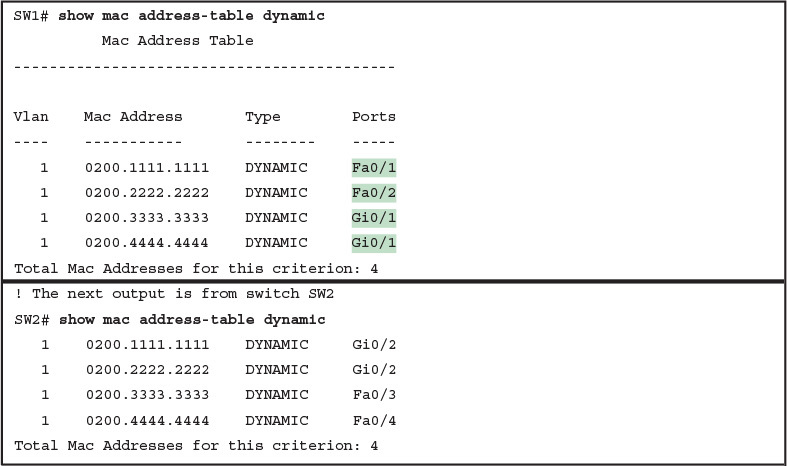
Example 8: The MAC Address Table on Two Switches

Using the Command-Line Interface
INTERNOLD NETWORKS CCNA LIVE WEBCLASS (INCLW)
Using the Command-Line Interface
Contents
Using the Command-Line Interface
To create an Ethernet LAN, a network engineer starts by planning. They consider the requirements, create a design, buy the switches, contract to install cables, and configure the switches to use the right features.
The CCNA Routing and Switching exams focus on skills like understanding how LANs work, configuring different switch features, verifying that those features work correctly, and finding the root cause of the problem when a feature is not working correctly.
The first skill you need to learn before doing all the configuration, verification, and troubleshooting tasks is to learn how to access and use the user interface of the switch, called the command-line interface (CLI).
This lesson begins that process by showing the basics of how to access the switch’s CLI. These skills include how to access the CLI and how to issue verification commands to check on the status of the LAN. This lesson also includes the processes of how to configure the switch and how to save that configuration.
Accessing the Cisco Catalyst Switch CLI
Cisco uses the concept of a command-line interface (CLI) with its router products and most of its Catalyst LAN switch products.
The CLI is a text-based interface in which the user, typically a network engineer, enters a text command and presses Enter.
Pressing Enter sends the command to the switch, which tells the device to do something. The switch does what the command says, and in some cases, the switch replies with some messages stating the results of the command.
Cisco Catalyst switches also support other methods to both monitor and configure a switch.
For example, a switch can provide a web interface, so that an engineer can open a web browser to connect to a web server running in the switch. Switches also can be controlled and operated using network management software.
This material discusses only Cisco Catalyst enterprise-class switches, and in particular, how to use the Cisco CLI to monitor and control these switches.
This first major section of the lesson first examines these Catalyst switches in more detail, and then explains how a network engineer can get access to the CLI to issue commands.
Cisco Catalyst Switches
Within the Cisco Catalyst brand of LAN switches, Cisco produces a wide variety of switch series or families.
Each switch series includes several specific models of switches that have similar features, similar price-versus-performance trade-offs, and similar internal components.
For example, the Cisco 2960-X series of switches. Cisco positions the 2960-X series (family) of switches as full-featured, low-cost wiring closet switches for enterprises. That means that you would expect to use 2960-X switches as access switches in a typical campus LAN design.
Figure 1 shows a photo of 10 different models from the 2960-X switch model series from Cisco.
Each switch series includes several models, with a mix of features.
For example, some of the switches have 48 RJ-45 unshielded twisted-pair (UTP) 10/100/1000 ports, meaning that these ports can autonegotiate the use of 10BASE-T (10 Mbps), 100BASE-T (100 Mbps), or 1000BASE-T (1 Gbps) Ethernet.

Figure 1: Cisco 2960-X Catalyst Switch Series
Accessing the Cisco IOS CLI
Like any other piece of computer hardware, Cisco switches need some kind of operating system software.
Cisco calls this OS the Internetwork Operating System (IOS).
Cisco IOS Software for Catalyst switches implements and controls logic and functions performed by a Cisco switch.
Besides controlling the switch’s performance and behavior, Cisco IOS also defines an interface for humans called the CLI.
The Cisco IOS CLI allows the user to use a terminal emulation program, which accepts text entered by the user. When the user presses Enter, the terminal emulator sends that text to the switch. The switch processes the text as if it is a command, does what the command says, and sends text back to the terminal emulator.
The switch CLI can be accessed through three popular methods—the console, Telnet, and Secure Shell (SSH).
Two of these methods (Telnet and SSH) use the IP network in which the switch resides to reach the switch. The console is a physical port built specifically to allow access to the CLI.
Figure 2 depicts the options.

Figure 2: CLI Access Options
Console access requires both a physical connection between a PC (or other user device) and the switch’s console port, as well as some software on the PC.
Telnet and SSH require software on the user’s device, but they rely on the existing TCP/IP network to transmit data.
The next few topics detail how to connect the console and set up the software for each method to access the CLI.
Cabling the Console Connection
The physical console connection, both old and new, uses three main components: the physical console port on the switch, a physical serial port on the PC, and a cable that works with the console and serial ports.
However, the physical cabling details have changed slowly over time, mainly because of advances and changes with serial interfaces on PC hardware.
For this next topic, the text looks at three cases: newer connectors on both the PC and the switch, older connectors on both, and a third case with the newer (USB) connector on the PC but with an older connector on the switch.
More modern PC and switch hardware use a familiar standard USB cable for the console connection. Cisco has been including USB ports as console ports in newer routers and switches as well.
All you have to do is look at the switch to make sure you have the correct style of USB cable end to match the USB console port. In the simplest form, you can use any USB port on the PC, with a USB cable, connected to the USB console port on the switch or router, as shown on the far right side of Figure 3.

Figure 3: Console Connection to a Switch
Older console connections use a PC serial port that pre-dates USB, a UTP cable, and an RJ-45 console port on the switch, as shown on the left side of Figure 3.
The PC serial port typically has a D-shell connector (roughly rectangular) with nine pins (often called a DB-9). The console port looks like any Ethernet RJ-45 port (but is typically colored in blue and with the word “console” beside it on the switch).
The cabling for this older-style console connection can be simple or require some effort, depending on what cable you use. You can use the purpose-built console cable that ships with new Cisco switches and routers and not think about the details.
However, you can make your own cable with a standard serial cable (with a connector that matches the PC), a standard RJ-45 to DB-9 converter plug, and a UTP cable.
However, the UTP cable does not use the same pinouts as Ethernet; instead, the cable uses rollover cable pinouts rather than any of the standard Ethernet cabling pinouts.
The rollover pinout uses eight wires, rolling the wire at pin 1 to pin 8, pin 2 to pin 7, pin 3 to pin 6, and so on.
As it turns out, USB ports became common on PCs before Cisco began commonly using USB for its console ports. So, you also have to be ready to use a PC that has only a USB port and not an old serial port, but a router or switch that has the older RJ-45 console port (and no USB console port).
The center of Figure 3 shows that case. To connect such a PC to a router or switch console, you need a USB converter that converts from the older console cable to a USB connector, and a rollover UTP cable, as shown in the middle of Figure 3.
NOTE: When using the USB options, you typically also need to install a software driver so that your PC’s OS knows that the device on the other end of the USB connection is the console of a Cisco device. Also, you can easily find photos of these cables and components online, with searches like “cisco console cable,” “cisco usb console cable,” or “console cable converter.”
The newer 2960-X series, for instance, supports both the older RJ-45 console port and a USB console port.
Figure 4 points to the two console ports; you would use only one or the other. Note that the USB console port uses a mini-B port rather than the more commonly seen rectangular standard USB port.

Figure 4: A Part of a 2960-X Switch with Console Ports Shown
After the PC is physically connected to the console port, a terminal emulator software package must be installed and configured on the PC.
The terminal emulator software treats all data as text. It accepts the text typed by the user and sends it over the console connection to the switch. Similarly, any bits coming into the PC over the console connection are displayed as text for the user to read.
The emulator must be configured to use the PC’s serial port to match the settings on the switch’s console port settings. The default console port settings on a switch are as follows.
Note that the last three parameters are referred to collectively as 8N1:
- 9600 bits/second
- No hardware flow control
- 8-bit ASCII
- No parity bits
- 1 stop bit
Figure 5 shows one such terminal emulator. The image shows the window created by the emulator software in the background, with some output of a show command.
The foreground, in the upper left, shows a settings window that lists the default console settings as listed just before this paragraph.

Figure 5: Terminal Settings for Console Access
Accessing the CLI with Telnet and SSH
For many years, terminal emulator applications have supported far more than the ability to communicate over a serial port to a local device (like a switch’s console).
Terminal emulators support a variety of TCP/IP applications as well, including Telnet and SSH.
Telnet and SSH both allow the user to connect to another device’s CLI, but instead of connecting through a console cable to the console port, the traffic flows over the same IP network that the networking devices are helping to create.
Telnet uses the concept of a Telnet client (the terminal application) and a Telnet server (the switch in this case). A Telnet client, the device that sits in front of the user, accepts keyboard input and sends those commands to the Telnet server.
The Telnet server accepts the text, interprets the text as a command, and replies back. Telnet is a TCP-based application layer protocol that uses well-known port 23.
Cisco Catalyst switches enable a Telnet server by default, but switches need a few more configuration settings before you can successfully use Telnet to connect to a switch. Chapter 8 covers switch configuration to support Telnet and SSH in detail.
Using Telnet in a lab today makes sense, but Telnet poses a significant security risk in production networks. Telnet sends all data (including any username and password for login to the switch) as clear-text data. SSH gives us a much better option.
Think of SSH as the much more secure Telnet cousin. Outwardly, you still open a terminal emulator, connect to the switch’s IP address, and see the switch CLI, no matter whether you use Telnet or SSH.
The differences exist behind the scenes: SSH encrypts the contents of all messages, including the passwords, avoiding the possibility of someone capturing packets in the network and stealing the password to network devices. Like Telnet, SSH uses TCP, just using well-known port 22 instead of Telnet’s 23.
User and Enable (Privileged) Modes
All three CLI access methods covered so far (console, Telnet, and SSH) place the user in an area of the CLI called user EXEC mode.
User EXEC mode, sometimes also called user mode, allows the user to look around but not break anything.
The “EXEC mode” part of the name refers to the fact that in this mode, when you enter a command, the switch executes the command and then displays messages that describe the command’s results.
Password Security for CLI Access from the Console
Cisco IOS supports a more powerful EXEC mode called enable mode (also known as privileged mode or privileged EXEC mode).
Enable mode gets its name from the enable command, which moves the user from user mode to enable mode, as shown in Figure 6.
The other name for this mode, privileged mode, refers to the fact that powerful (or privileged) commands can be executed there. For example, you can use the reload command, which tells the switch to reinitialize or reboot Cisco IOS, only from enable mode.

Figure 6: User and Privileged Modes
NOTE: If the command prompt lists the hostname followed by a >, the user is in user mode; if it is the hostname followed by the #, the user is in enable mode.
Example 1 demonstrates the differences between user and enable modes.
The example shows the output that you could see in a terminal emulator window, for instance, when connecting from the console.
In this case, the user sits at the user mode prompt (“Certskills1>”) and tries the reload command.
The reload command tells the switch to reinitialize or reboot Cisco IOS, so IOS allows this powerful command to be used only from enable mode.
IOS rejects the reload command when used in user mode. Then the user moves to enable mode—also called privileged mode—(using the enable EXEC command).
At that point, IOS accepts the reload command now that the user is in enable mode.

Example 1: Privileged Mode Commands Being Rejected in User Mode
NOTE:
The commands that can be used in either user (EXEC) mode or enable (EXEC) mode are called EXEC commands.
This example is the first instance of this lesson showing you the output from the CLI, so it is worth noting a few conventions.
The bold text represents what the user typed, and the nonbold text is what the switch sent back to the terminal emulator.
Also, the typed passwords do not show up on the screen for security purposes.
Finally, note that this switch has been preconfigured with a hostname of Certskills1, so the command prompt on the left shows that hostname on each line.
Password Security for CLI Access from the Console
A Cisco switch, with default settings, remains relatively secure when locked inside a wiring closet, because by default, a switch allows console access only.
By default, the console requires no password at all, and no password to reach enable mode for users that happened to connect from the console.
The reason is that if you have access to the physical console port of the switch, you already have pretty much complete control over the switch.
You could literally get out your screwdriver and walk off with it, or you could unplug the power, or follow well-published procedures to go through password recovery to break into the CLI and then configure anything you want to configure.
However, many people go ahead and set up simple password protection for console users.
Simple passwords can be configured at two points in the login process from the console: when the user connects from the console, and when any user moves to enable mode (using the enable EXEC command).
You may have noticed that back in Example 1, the user saw a password prompt at both points.
Example 2 shows the additional configuration commands that were configured prior to collecting the output in Example 1. The output holds an excerpt from the EXEC command show running-config, which lists the current configuration in the switch.

Example 2: Nondefault Basic Configuration
Working from top to bottom, note that the first configuration command listed by the show running-config command sets the switch’s hostname to Certskills1.
You might have noticed that the command prompts in Example 1 all began with Certskills1, and that’s why the command prompt begins with the hostname of the switch.
Next, note that the lines with a ! in them are comment lines, both in the text of this book and in the real switch CLI.
The enable secret love configuration command defines the password that all users must use to reach enable mode. So, no matter whether a user connects from the console, Telnet, or SSH, they would use password love when prompted for a password after typing the enable EXEC command.
Finally, the last three lines configure the console password. The first line (line console 0) is the command that identifies the console, basically meaning “these next commands apply to the console only.” The login command tells IOS to perform simple password checking (at the console).
Remember, by default, the switch does not ask for a password for console users. Finally, the password faith command defines the password the console user must type when prompted.
This example just scratches the surface of the kinds of security configuration you might choose to configure on a switch, but it does give you enough detail to configure switches in your lab and get started.
Note that there will be lesson that shows the configuration steps to add support for Telnet and SSH (including password security).
CLI Help Features
If you printed the Cisco IOS Command Reference documents, you would end up with a stack of paper several feet tall.
No one should expect to memorize all the commands—and no one does. You can use several very easy, convenient tools to help remember commands and save time typing.
As you progress through your Cisco certifications, the exams will cover progressively more commands. However, you should know the methods of getting command help.
Table 1 summarizes command-recall help options available at the CLI.
Note that, in the first column, command represents any command. Likewise, parm represents a command’s parameter.
For example, the third row lists command ?, which means that commands such as show ? and copy ? would list help for the show and copy commands, respectively.

Table 1: Cisco IOS Software Command Help
When you enter the ?, the Cisco IOS CLI reacts immediately; that is, you don’t need to press the Enter key or any other keys.
The device running Cisco IOS also redisplays what you entered before the ? to save you some keystrokes. If you press Enter immediately after the ?, Cisco IOS tries to execute the command with only the parameters you have entered so far.
The information supplied by using help depends on the CLI mode. For example, when ? is entered in user mode, the commands allowed in user mode are displayed, but commands available only in enable mode (not in user mode) are not displayed.
Also, help is available in configuration mode, which is the mode used to configure the switch. In fact, configuration mode has many different subconfiguration modes, as explained in the section “Configuration Submodes and Contexts,” later in this chapter.
So, you can get help for the commands available in each configuration submode as well.
Cisco IOS stores the commands that you enter in a history buffer, storing ten commands by default. The CLI allows you to move backward and forward in the historical list of commands and then edit the command before reissuing it.
These key sequences can help you use the CLI more quickly on the exams.
Table 2 lists the commands used to manipulate previously entered commands.

Table 2: Key Sequences for Command Edit and Recall
The debug and show Commands
By far, the single most popular Cisco IOS command is the show command.
The show command has a large variety of options, and with those options, you can find the status of almost every feature of Cisco IOS.
Essentially, the show command lists the currently known facts about the switch’s operational status. The only work the switch does in reaction to show commands is to find the current status and list the information in messages sent to the user.
For example, consider the output from the show mac address-table dynamic command listed in Example 3.
This show command, issued from user mode, lists the table the switch uses to make forwarding decisions. A switch’s MAC address table basically lists the data a switch uses to do its primary job.

Example 3: Nondefault Basic Configuration
The debug command also tells the user details about the operation of the switch. However, while the show command lists status information at one instant of time—more like a photograph—the debug command acts more like a live video camera feed.
Once you issue a debug command, IOS remembers, issuing messages that any switch user can choose to see. The console sees these messages by default.
Most of the commands used throughout this book to verify operation of switches and routers are show commands.
Configuring Cisco IOS Software
You will want to configure every switch in an Enterprise network, even though the switches will forward traffic even with default configuration.
This section covers the basic configuration processes, including the concept of a configuration file and the locations in which the configuration files can be stored.
Although this section focuses on the configuration process, and not on the configuration commands themselves, you should know all the commands covered in this chapter for the exams, in addition to the configuration processes.
Configuration mode is another mode for the Cisco CLI, similar to user mode and privileged mode. User mode lets you issue non-disruptive commands and displays some information.
Privileged mode supports a superset of commands compared to user mode, including commands that might disrupt switch operations.
However, none of the commands in user or privileged mode changes the switch’s configuration. Configuration mode accepts configuration commands—commands that tell the switch the details of what to do and how to do it.
Figure 7 illustrates the relationships among configuration mode, user EXEC mode, and privileged EXEC mode.

Figure 7: CLI Configuration Mode Versus EXEC Modes
Commands entered in configuration mode update the active configuration file. These changes to the configuration occur immediately each time you press the Enter key at the end of a command. Be careful when you enter a configuration command!
Configuration Submodes and Contexts
Configuration mode itself contains a multitude of commands. To help organize the configuration, IOS groups some kinds of configuration commands together.
To do that, when using configuration mode, you move from the initial mode—global configuration mode—into subcommand modes. Context-setting commands move you from one configuration subcommand mode, or context, to another.
These context-setting commands tell the switch the topic about which you will enter the next few configuration commands.
More importantly, the context tells the switch the topic you care about right now, so when you use the ? to get help, the switch gives you help about that topic only.
NOTE: Context-setting is not a Cisco term. It is just a description used here to help make sense of configuration mode.
The best way to learn about configuration submodes is to use them, but first, take a look at these upcoming examples.
For instance, the interface command is one of the most commonly used context-setting configuration commands.
For example, the CLI user could enter interface configuration mode by entering the interface FastEthernet 0/1 configuration command. Asking for help in interface configuration mode displays only commands that are useful when configuring Ethernet interfaces.
Commands used in this context are called subcommands—or, in this specific case, interface subcommands.
When you begin practicing with the CLI with real equipment (or simulation), the navigation between modes can become natural. For now, consider Example 4, which shows the following:
- Movement from enable mode to global configuration mode by using the configure terminal EXEC command.
- Using a hostname Fred global configuration command to configure the switch’s name.
- Movement from global configuration mode to console line configuration mode (using the line console 0 command).
- Setting the console’s simple password to hope (using the password hope line subcommand).
- Movement from console configuration mode to interface configuration mode (using the interface type number command).
- Setting the speed to 100 Mbps for interface Fa0/1 (using the speed 100 interface subcommand).
- Movement from interface configuration mode back to global configuration mode (using the exit command).

Example 4: Navigating Between Different Configuration Modes
The text inside parentheses in the command prompt identifies the configuration mode. For example, the first command prompt after you enter configuration mode lists (config), meaning global configuration mode.
After the line console 0 command, the text expands to (config-line), meaning line configuration mode. Each time the command prompt changes within config mode, you have moved to another configuration mode.
Table 3 shows the most common command prompts in configuration mode, the names of those modes, and the context-setting commands used to reach those modes.

Table 3: Common Switch Configuration Modes
You should practice until you become comfortable moving between the different configuration modes, back to enable mode, and then back into the configuration modes.
However, you can learn these skills just doing labs about the topics in later lessons.
For now, Figure 8 shows most of the navigation between global configuration mode and the four configuration submodes listed in Table 3.

Figure 8: Navigation In and Out of Switch Configuration Modes
NOTE: You can also move directly from one configuration submode to another, without first using the exit command to move back to global configuration mode. Just use the commands listed in bold in the center of the figure.
You really should stop and try navigating around these configuration modes.
No set rules exist for what commands are global commands or subcommands.
Generally, however, when multiple instances of a parameter can be set in a single switch, the command used to set the parameter is likely a configuration subcommand.
Items that are set once for the entire switch are likely global commands. For example, the hostname command is a global command because there is only one hostname per switch.
Conversely, the speed command is an interface subcommand that applies to each switch interface that can run at different speeds, so it is a subcommand, applying to the particular interface under which it is configured.
Storing Switch Configuration Files
When you configure a switch, it needs to use the configuration. It also needs to be able to retain the configuration in case the switch loses power.
Cisco switches contain random-access memory (RAM) to store data while Cisco IOS is using it, but RAM loses its contents when the switch loses power or is reloaded.
To store information that must be retained when the switch loses power or is reloaded, Cisco switches use several types of more permanent memory, none of which has any moving parts.
By avoiding components with moving parts (such as traditional disk drives), switches can maintain better uptime and availability.
The following list details the four main types of memory found in Cisco switches, as well as the most common use of each type:
- RAM: Sometimes called DRAM, for dynamic random-access memory, RAM is used by the switch just as it is used by any other computer: for working storage. The running (active) configuration file is stored here.
- Image Flash memory: Either a chip inside the switch or a removable memory card, flash memory stores fully functional Cisco IOS images and is the default location where the switch gets its Cisco IOS at boot time. Flash memory also can be used to store any other files, including backup copies of configuration files.
- ROM: Read-only memory (ROM) stores a bootstrap (or boothelper) program that is loaded when the switch first powers on. This bootstrap program then finds the full Cisco IOS image and manages the process of loading Cisco IOS into RAM, at which point Cisco IOS takes over operation of the switch.
- NVRAM: Nonvolatile RAM (NVRAM) stores the initial or startup configuration file that is used when the switch is first powered on and when the switch is reloaded.
Figure 9 summarizes this same information in a briefer and more convenient form for memorization and study.

Figure 9: Cisco Switch Memory Types
Cisco IOS stores the collection of configuration commands in a configuration file. In fact, switches use multiple configuration files—one file for the initial configuration used when powering on, and another configuration file for the active, currently used running configuration as stored in RAM.
Table 4 lists the names of these two files, their purpose, and their storage location.

Table 4: Names and Purposes of the Two Main Cisco IOS Configuration Files
Essentially, when you use configuration mode, you change only the running-config file. This means that the configuration example earlier in this chapter (Example 4) updates only the running-config file.
However, if the switch lost power right after that example, all that configuration would be lost. If you want to keep that configuration, you have to copy the running-config file into NVRAM, overwriting the old startup-config file.
Example 5 demonstrates that commands used in configuration mode change only the running configuration in RAM. The example shows the following concepts and steps:
- Step 1. The example begins with both the running and startup-config having the same hostname, per the hostname hannah command.
- Step 2. The hostname is changed in configuration mode using the hostname jessie command.
- Step 3. The show running-config and show startup-config commands show the fact that the hostnames are now different, with the hostname jessie command found only in the running-config.

Example 5: How Configuration Mode Commands Change the Running-Config File, Not the Startup-Config File
Copying and Erasing Configuration Files
The configuration process updates the running-config file, which is lost if the router loses power or is reloaded.
Clearly, IOS needs to provide us a way to copy the running configuration so that it will not be lost, so it will be used the next time the switch reloads or powers on.
For instance, Example 5 ended with a different running configuration (with the hostname jessie command) versus the startup configuration.
In short, the EXEC command copy running-config startup-config backs up the running-config to the startup-config file. This command overwrites the current startup-config file with what is currently in the running-configuration file.
In addition, in lab, you may want to just get rid of all existing configuration and start over with a clean configuration. To do that, you can erase the startup-config file using three different commands:
write erase
erase startup-config
erase nvram:
Once the startup-config file is erased, you can reload or power off/on the switch, and it will boot with the now-empty startup configuration.
Note that Cisco IOS does not have a command that erases the contents of the running-config file. To clear out the running-config file, simply erase the startup-config file, and then reload the switch, and the running-config will be empty at the end of the process.
NOTE: Cisco uses the term reload to refer to what most PC operating systems call rebooting or restarting. In each case, it is a re-initialization of the software. The reload EXEC command causes a switch to reload.

How To
INTERNOLD NETWORKS CCNA LIVE WEBCLASS (INCLW)
HOW TO
How To Download .ovpn File Using WinSCP
How To Access Modules and Resources

Template Module 1
Fundamentals of ethernet lans and wanS
VIDEO LESSONS
Overview of LANs (SOHO and Enterprise LANs)
Blank
Blank
Blank
Fundamentals of Ethernet LANs and WANs – Clone
Fundamentals of ethernet lans and wanS
VIDEO LESSONS
Overview of LANs (SOHO and Enterprise LANs) - 2 videos
Building Physical Ethernet Networks with UTP (1 video)
Sending Data in Ethernet Networks (4 videos)
RESOURCES
Template Module
Fundamentals of TCP/IP Networking
VIDEO LESSONS
Perspectives on Networking (1 video)
TCP/IP Networking Model (3 videos)
TCP/IP Model Layers (3 videos)
OSI Networking Model (2 videos)


Fundamentals of IPv4 Addressing and Routing – Detailed Discussion
INTERNOLD NETWORKS CCNA LIVE WEBCLASS (INCLW)
Fundamentals of IPv4 Addressing and Routing
Contents
Fundamentals of IPv4 Addressing and Routing
The TCP/IP network layer (Layer 3) defines how to deliver IP packets over the entire trip, from the original device that creates the packet to the device that needs to receive the packet.
That process requires cooperation among several different jobs and concepts on a number of devices.
- IP routing: The process of hosts and routers forwarding IP packets (Layer 3 protocol data units [PDU]), while relying on the underlying LANs and WANs to forward the bits.
- IP addressing: Addresses used to identify a packet’s source and destination host computer. Addressing rules also organize addresses into groups, which greatly assists the routing process.
- IP routing protocol: A protocol that aids routers by dynamically learning about the IP address groups so that a router knows where to route IP packets so that they go to the right destination host.
- Other utilities: The network layer also relies on other utilities. For TCP/IP, these utilities include Domain Name System (DNS), Address Resolution Protocol (ARP), and ping.
Note that all these functions have variations both for the well-established IP version 4 (IPv4) and for the emerging newer IP version 6 (IPv6).
Overview of Network Layer Functions
Many protocol models have existed over the years, but today the TCP/IP model dominates.
And at the network layer of TCP/IP, two options exist for the main protocol around which all other network layer functions revolve: IP version 4 (IPv4) and IP version 6 (IPv6).
Both IPv4 and IPv6 define the same kinds of network layer functions, but with different details.
IP focuses on the job of routing data, in the form of IP packets, from the source host to the destination host.
IP does not concern itself with the physical transmission of data, instead relying on the lower TCP/IP layers to do the physical transmission of the data.
Instead, IP concerns itself with the logical details, rather than physical details, of delivering data.
In particular, the network layer specifies how packets travel end to end over a TCP/IP network, even when the packet crosses many different types of LAN and WAN links.
Network Layer Routing (Forwarding) Logic
Routers and end-user computers (called hosts in a TCP/IP network) work together to perform IP routing.
The host operating system (OS) has TCP/IP software, including the software that implements the network layer.
Hosts use that software to choose where to send IP packets, often to a nearby router. Those routers make choices of where to send the IP packet next.
Together, the hosts and routers deliver the IP packet to the correct destination, as shown in the example in the diagram below.

Routing Logic: PC1 Sending an IP Packet to PC2
The IP packet, created by PC1, goes from the top of the figure all the way to PC2 at the bottom of the figure.
NOTE: The term path selection is sometimes used to refer to the routing process shown in previous diagram. At other times, it refers to routing protocols, specifically how routing protocols select the best route among the competing routes to the same destination.
Host Forwarding Logic: Send the Packet to the Default Router
In prior diagram, PC1 does some basic analysis, and then chooses to send the IP packet to the router so that the router will forward the packet.
PC1 analyzes the destination address and realizes that PC2’s address (168.1.1.1) is not on the same LAN as PC1.
So PC1’s logic tells it to send the packet to a device whose job it is to know where to route data: a nearby router, on the same LAN, called PC1’s default router.
To send the IP packet to the default router, the sender sends a data-link frame across the medium to the nearby router; this frame includes the packet in the data portion of the frame.
That frame uses data link layer (Layer 2) addressing in the data-link header to ensure that the nearby router receives the frame.
NOTE: The default router is also referred to as the default gateway.
R1 and R2’s Logic: Routing Data Across the Network
All routers use the same general process to route the packet.
Each router keeps an IP routing table. This table lists IP address groupings, called IP networks and IP subnets.
When a router receives a packet, it compares the packet’s destination IP address to the entries in the routing table and makes a match. This matching entry also lists directions that tell the router where to forward the packet next.
In the above diagram, R1 would have matched the destination address (168.1.1.1) to a routing table entry, which in turn told R1 to send the packet to R2 next.
Similarly, R2 would have matched a routing table entry that told R2 to send the packet, over an Ethernet over MPLS (EoMPLS) link, to R3 next.
The routing concept works a little like driving down the freeway when approaching a big interchange. You look up and see signs for nearby towns, telling you which exits to take to go to each town.
Similarly, the router looks at the IP routing table (the equivalent of the road signs) and directs each packet over the correct next LAN or WAN link (the equivalent of a road).
R3’s Logic: Delivering Data to the End Destination
The final router in the path, R3, uses almost the same logic as R1 and R2, but with one minor difference. R3 needs to forward the packet directly to PC2, not to some other router.
How Network Layer Routing Uses LANs and WANs
While the network layer routing logic ignores the physical transmission details, the bits still have to be transmitted.
To do that work, the network layer logic in a host or router must hand off the packet to the data link layer protocols, which, in turn, ask the physical layer to actually send the data.
The data link layer adds the appropriate header and trailer to the packet, creating a frame, before sending the frames over each physical network.
The routing process forwards the network layer packet from end to end through the network, while each data-link frame only takes a smaller part of the trip.
Each successive data link layer frame moves the packet to the next device that thinks about network layer logic.
In short, the network layer thinks about the bigger view of the goal, like “Send this packet to the specified next device...,” while the data link layer thinks about the specifics, like “Encapsulate the packet in a data-link frame and transmit it.”
The diagram below points out the key encapsulation logic on each device.

Network Layer and Data Link Layer Encapsulation
Because the routers build new data-link headers and trailers, and because the new headers contain data-link addresses, the PCs and routers must have some way to decide what data-link addresses to use.
An example of how the router determines which data-link address to use is the IP Address Resolution Protocol (ARP). ARP dynamically learns the data-link address of an IP host connected to a LAN.
For example, at the last step, at the bottom of above diagram, Router R3 would use ARP once to learn PC2’s MAC address before sending any packets to PC2.
Routing as covered so far has two main concepts:
- The process of routing forwards Layer 3 packets, also called Layer 3 protocol data units (L3 PDU), based on the destination Layer 3 address in the packet.
- The routing process uses the data link layer to encapsulate the Layer 3 packets into Layer 2 frames for transmission across each successive data link.
IP Addressing and How Addressing Helps IP Routing
IP defines network layer addresses that identify any host or router interface that connects to a TCP/IP network.
The idea basically works like a postal address: Any interface that expects to receive IP packets needs an IP address, just like you need a postal address before receiving mail from the postal service.
TCP/IP groups IP addresses together so that IP addresses used on the same physical network are part of the same group.
IP calls these address groups an IP network or an IP subnet.
Using that same postal service analogy, each IP network and IP subnet works like a postal code (or ZIP code). All nearby postal addresses are in the same postal code (ZIP code), while all nearby IP addresses must be in the same IP network or IP subnet.
IP defines specific rules about which IP address should be in the same IP network or IP subnet.
Numerically, the addresses in the same group have the same value in the first part of the addresses.
For example, the previous diagrams could have used the following conventions:
- Hosts on the top Ethernet: Addresses start with 10
- Hosts on the R1-R2 serial link: Addresses start with 168.10
- Hosts on the R2-R3 EoMPLS link: Addresses start with 168.11
- Hosts on the bottom Ethernet: Addresses start with 168.1
To make routing more efficient, network layer protocols group addresses, both by their location and by the actual address values. A router can list one routing table entry for each IP network or subnet, instead of one entry for every single IP address.
The routing process also makes use of a 20-byteIPv4 header, as shown in below diagram.
The header lists a 32-bit source IP address, as well as a 32-bit destination IP address.

IPv4 Header, Organized as Four Bytes Wide for a Total of 20 Bytes
Routing Protocols
For routing logic to work on both hosts and routers, each needs to know something about the TCP/IP internetwork.
Hosts need to know the IP address of their default router so that hosts can send packets to remote destinations.
Routers, however, need to know routes so that routers know how to forward packets to each and every IP network and IP subnet.
Although a network engineer could configure (type) all the required routes, on every router, most network engineers instead simply enable a routing protocol on all routers.
If you enable the same routing protocol on all the routers in a TCP/IP internetwork, with the correct settings, the routers will send routing protocol messages to each other.
As a result, all the routers will learn routes for all the IP networks and subnets in the TCP/IP internetwork.
Diagram below shows an example.

Example of How Routing Protocols Advertise About Networks and Subnets
In this case, IP network 168.1.0.0, which consists of all addresses that begin with 168.1, sits on the Ethernet at the bottom of the diagram.
R3, knowing this fact, sends a routing protocol message to R2 (Step 1).
R2 learns a route for network 168.1.0.0 as a result, as shown on the left.
At Step 2, R2 turns around and sends a routing protocol message to R1 so that R1 now has a route for that same IP network (168.1.0.0).
IPv4 Addressing
One of the most important concept in your CCNA study is the understanding of IP addresses, their formats, the grouping concepts, how to subdivide groups into subnets, how to interpret the documentation for existing networks’ IP addressing, and so on.
Simply put, you had better know addressing and subnetting!
Rules for IP Addresses
If a device wants to communicate using TCP/IP, it needs an IP address.
When the device has an IP address and the appropriate software and hardware, it can send and receive IP packets.
Any device that has at least one interface with an IP address can send and receive IP packets and is called an IP host.
IP addresses consist of a 32-bit number, usually written in dotted-decimal notation (DDN).
The “decimal” part of the term comes from the fact that each byte (8 bits) of the 32-bit IP address is shown as its decimal equivalent.
The four resulting decimal numbers are written in sequence, with “dots,” or decimal points, separating the numbers—hence the name dotted-decimal.
For example, 168.1.1.1 is an IP address written in dotted-decimal form; the actual binary version is 10101000 00000001 00000001 00000001.
Each DDN has four decimal octets, separated by periods. The term octet is just a vendor-neutral term for byte.
Because each octet represents an 8-bit binary number, the range of decimal numbers in each octet is between 0 and 255, inclusive.
For example, the IP address of 168.1.1.1 has a first octet of 168, the second octet of 1, and so on.
Finally, note that each network interface uses a unique IP address. Most people tend to think that their computer has an IP address, but actually their computer’s network card has an IP address.
For example, if your laptop has both an Ethernet network interface card (NIC) and a wireless NIC, with both working at the same time, both will have an IP address.
Similarly, routers, which typically have many network interfaces that forward IP packets, have an IP address for each interface.
Rules for Grouping IP Addresses
The original specifications for TCP/IP grouped IP addresses into sets of consecutive addresses called IP networks.
The addresses in a single IP network have the same numeric value in the first part of all addresses in the network.
The diagram below shows a simple internetwork that has three separate IP networks.

Sample TCP/IP Internetwork Using IPv4 Network Numbers
The diagram lists a network identifier (network ID) for each network, as well as a text description of the DDN values in each network.
For example, the hosts in the Ethernet LAN on the far left use IP addresses that begin with a first octet of 8; the network ID happens to be 8.0.0.0.
As another example, the serial link between R1 and R2 consists of only two interfaces—a serial interface on each router—and uses an IP address that begins with the three octets 199.1.1.
The above diagram also provides a good figure with which to discuss two important facts about how IPv4 groups IP addresses:
- All IP addresses in the same group must not be separated from each other by a router.
- IP addresses separated from each other by a router must be in different groups.
Take the first of the two rules, and look at hosts A and B on the left.
Hosts A and B are in the same IP network and have IP addresses that begin with 8.
Per the first rule, hosts A and B cannot be separated from each other by a router (and they are indeed not separated from each other by a router).
Next, take the second of the two rules and add host C to the discussion. Host C is separated from host A by at least one router, so host C cannot be in the same IP network as host A. Host C’s address cannot begin with 8.
Likewise, IP routing relies on all addresses in one IP network or IP subnet being in the same location, specifically on a single instance of a LAN or WAN data link. Otherwise, the routers might deliver IP packets to the wrong locations.
For any TCP/IP internetwork, each LAN and WAN link will use either an IP network or an IP subnet.
Class A, B, and C IP Networks
The IPv4 address space includes all possible combinations of numbers for a 32-bit IPv4 address.
Literally 232 different values exist with a 32-bit number, for more than 4 billion different numbers.
With DDN values, these numbers include all combinations of the values 0 through 255 in all four octets: 0.0.0.0, 0.0.0.1, 0.0.0.2, and all the way up to 255.255.255.255.
IP standards first subdivide the entire address space into classes, as identified by the value of the first octet.
- Class A gets roughly half of the IPv4 address space, with all DDN numbers that begin with 1–126..
- Class B gets one-fourth of the address space, with all DDN numbers that begin with 128–191 inclusive.
- Class C gets one-eighth of the address space, with all numbers that begin with 192–223.
See diagram below for details.

Division of the Entire IPv4 Address Space by Class
The diagram also notes the purpose for the five address classes.
- Classes A, B, and C define unicast IP addresses, meaning that the address identifies a single host interface.
- Class D defines multicast addresses, used to send one packet to multiple hosts.
- Class E originally defined experimental addresses but are now reserved for future use.
IPv4 standards also subdivide the Class A, B, and C unicast classes into predefined IP networks.
Each IP network makes up a subset of the DDN values inside the class.
IPv4 uses three classes of unicast addresses so that the IP networks in each class can be different sizes, and therefore meet different needs.
Class A networks each support a very large number of IP addresses (more than 16 million host addresses per IP network).
However, because each Class A network is so large, Class A holds only 126 Class A networks.
Class B defines IP networks that have 65,534 addresses per network, but with space for more than 16,000 such networks.
Class C defines much smaller IP networks, with 254 addresses each.
See the diagram below for details.

Size of Network and Host Parts of Class A, B, and C Addresses
The diagram shows a visual perspective, as well as the literal numbers, for all the Class A, B, and C IPv4 networks in the entire world. It shows clouds for IP networks.
It, of course, does not show one cloud for every possible network, but shows the general idea, with a small number of large clouds for Class A and a large number of small clouds for Class C.
The Actual Class A, B, and C IP Networks
The previous diagram shows the number of Class A, B, and C IP networks in the entire world.
Eventually, you need to actually pick and use some of these IP networks to build a working TCP/IP internetwork, so you need to be able to answer the question: What are the specific IP networks?
First, you must be able to identify each network briefly using a network identifier (network ID).
The network ID is just one reserved DDN value per network that identifies the IP network. (The network ID cannot be used by a host as an IP address.)
For example, the table shows the network IDs that match the given diagram.
Sample TCP/IP Internetwork Using IPv4 Network Numbers

Network IDs Used
NOTE: Many people use the term network ID, but others use the terms network number and network address. Be ready to use all three terms.
So, what are the actual Class A, B, and C IP networks, and what are their network IDs?
First, consider the Class A networks. As learned, only 126 Class A networks exist.
As it turns out, they consist of all addresses that begin with 1, all addresses that begin with 2, all addresses that begin with 3, and so on, up through the 126th such network of “all addresses that begin with 126.”
The table below lists a few of these networks.

Sampling of IPv4 Class A Networks
Class B networks have a first octet value between 128 and 191, inclusive, but in a single Class B network, the addresses have the same value in the first two octets.
For example, our previous diagram uses Class B network 130.4.0.0. The DDN value 130.4.0.0 must be in Class B, because the first octet is between 128 and 191, inclusive.
However, the first two octets define the addresses in a single Class B network.
Table below lists some sample IPv4 Class B networks.

Sampling of IPv4 Class B Networks
Class C networks can also be easily identified, with a first octet value between 192 and 223, inclusive.
With Class C networks and addresses, the first three octets define the group, with addresses in one Class C network having the same value in the first three octets.
Table below shows some samples.

Sampling of IPv4 Class C Networks
Listing all the Class A, B, and C networks would of course take too much space.
Table below summarizes the first octet values that identify the class and summarizes the range of Class A, B, and C network numbers available in the entire IPv4 address space.

All Possible Valid Network Numbers
NOTE: The term classful IP network refers to any Class A, B, or C network, because it is defined by Class A, B, and C rules.
IP Subnetting
Like IP addressing, IP subnetting is also one of the most important topics that a Network Engineer needs to master.
Subnetting defines methods of further subdividing the IPv4 address space into groups that are smaller than a single IP network.
IP subnetting defines a flexible way for anyone to take a single Class A, B, or C IP network and further subdivide it into even smaller groups of consecutive IP addresses.
In fact, the name subnet is just shorthand for subdivided network. Then, in each location where you used to use an entire Class A, B, or C network, you can use a smaller subnet, wasting fewer IP addresses.
To make it clear how an internetwork can use both classful IPv4 networks as well as subnets of classful IPv4 networks, the next two diagrams show the same internetwork, one with classful networks only and one with subnets only. The first diagram uses five Class B networks with no subnetting.
The design in 1st diagram below requires five groups of IP addresses, each of which is a Class B network in this example.
Specifically, the three LANs each use a single Class B network, and the two serial links each use a Class B network.
It wastes many IP addresses, because each Class B network has 216 – 2 host addresses—far more than you will ever need for each LAN and WAN link.
For example, the Ethernet on the left uses an entire Class B network, which supports 65,534 IP addresses that begin with 150.1.
However, a single LAN seldom grows past a few hundred devices, so many of the IP addresses in Class B network 150.1.0.0 would be wasted. Even more waste occurs on the point-to-point serial links, which need only two IP addresses.
The 2nd diagram illustrates a more common design today, one that uses basic subnetting. As in the previous diagram, it needs five groups of addresses.
However, in this case, the figure uses five subnets of Class B network 150.9.0.0.

Example That Uses Five Class B Networks

Using Subnets for the Same Design as the Previous Figure
Subnetting allows the network engineer for the TCP/IP internetwork to choose to use a longer part of the addresses that must have the same value.
Subnetting allows quite a bit of flexibility, but 2nd diagram above shows one of the simplest forms of subnetting.
In this case, each subnet includes the addresses that begin with the same value in the first three octets, as follows:
- One group of the 254 addresses that begin with 150.9.1
- One group of the 254 addresses that begin with 150.9.2
- One group of the 254 addresses that begin with 150.9.3
- One group of the 254 addresses that begin with 150.9.4
- One group of the 254 addresses that begin with 150.9.5
As a result of using subnetting, the network engineer has saved many IP addresses.
First, only a small part of Class B network 150.9.0.0 has been used so far. Each subnet has 254 addresses, which should be plenty of addresses for each LAN, and more than enough for the WAN links.
In summary, you now know some of the details of IP addressing, with a focus on how it relates to routing. Each host and router interface will have an IP address.
However, the IP addresses will not be randomly chosen but will instead be grouped together to aid the routing process.
The groups of addresses can be an entire Class A, B, or C network number or it can be a subnet.
IPv4 Routing
IPv4 Host Routing
Hosts actually use some simple routing logic when choosing where to send a packet. If you assume that the design uses subnets (which is typical), this two-step logic is as follows:
- Step 1. If the destination IP address is in the same IP subnet as I am, send the packet directly to that destination host.
- Step 2. Otherwise, send the packet to my default gateway, also known as a default router. (This router has an interface on the same subnet as the host.)
For example, consider the diagram below and focus on the Ethernet LAN on the left.

Host Routing: Forwarding to a Host on the Same Subnet
When PC1 sends an IP packet to PC11 (150.9.1.11), PC1 first considers some match related to subnetting.
PC1 concludes that PC11’s IP address is in the same subnet as PC1, so PC1 ignores its default router (Core, 150.9.1.1), sending the packet directly to PC11, as shown in Step 1 of the diagram.
Alternatively, when PC1 sends a packet to PC2 (150.9.4.10), PC1 does the same kind of subnetting math, and realizes that PC2 is not on the same subnet as PC1.
So, PC1 forwards the packet (Step 2) to its default gateway, 150.9.1.1, which then routes the packet to PC2.
Router Forwarding Decisions and the IP Routing Table
A Summary of Router Forwarding Logic
First, when a router receives a data-link frame addressed to that router’s data-link address, the router needs to think about processing the contents of the frame.
When such a frame arrives, the router uses the following logic on the data-link frame:
- Step 1. Use the data-link Frame Check Sequence (FCS) field to ensure that the frame had no errors; if errors occurred, discard the frame.
- Step 2. Assuming that the frame was not discarded at Step 1, discard the old data-link header and trailer, leaving the IP packet.
- Step 3. Compare the IP packet’s destination IP address to the routing table, and find the route that best matches the destination address. This route identifies the outgoing interface of the router, and possibly the next-hop router IP address.
- Step 4. Encapsulate the IP packet inside a new data-link header and trailer, appropriate for the outgoing interface, and forward the frame.
With these steps, each router forwards the packet to the next location, inside a data-link frame.
With each router repeating this process, the packet reaches its final destination.
While the router does all the steps in the list, Step 3 is the main routing or forwarding step.
The packet has a destination IP address in the header, whereas the routing table lists slightly different numbers, typically a list of networks and subnets.
To match a routing table entry, the router thinks like this:
- Network numbers and subnet numbers represent a group of addresses that begin with the same prefix.
- Think about those numbers as groups of addresses.
- In which of the groups does this packet’s destination address reside?
The next example shows specific examples of matching the routing table.
A Detailed Routing Example
The routing example uses the diagram below.
In this example, all routers happen to use the Open Shortest Path First (OSPF) routing protocol, and all routers know routes for all subnets.
In particular, PC2, at the bottom, sits in subnet 150.150.4.0, which consists of all addresses that begin with 150.150.4.
In the example, PC1 sends an IP packet to 150.150.4.10, PC2’s IP address.

Simple Routing Example, with IP Subnets
NOTE: Note that the routers all know in this case that “subnet 150.150.4.0” means “all addresses that begin with 150.150.4.”
The following list explains the forwarding logic at each step in the diagram above.
(Note that the text refers to Steps 1, 2, 3, and 4 of the routing logic shown in the previous section -- A Summary of Router Forwarding Logic)
- Step A
- PC1 sends the packet to its default router.
- PC1 first builds the IP packet, with a destination address of PC2’s IP address (150.150.4.10).
- PC1 needs to send the packet to R1 (PC1’s default router) because the destination address is on a different subnet.
- PC1 places the IP packet into an Ethernet frame, with a destination Ethernet address of R1’s Ethernet address.
- PC1 sends the frame on to the Ethernet. (Note that the figure omits the data-link trailers.)
- Step B
- R1 processes the incoming frame and forwards the packet to R2.
- Because the incoming Ethernet frame has a destination MAC of R1’s Ethernet MAC, R1 copies the frame off the Ethernet for processing.
- R1 checks the frame’s FCS, and no errors have occurred (Step 1).
- R1 then discards the Ethernet header and trailer (Step 2).
- Next, R1 compares the packet’s destination address (150.150.4.10) to the routing table and finds the entry for subnet 150.150.4.0—which includes addresses 150.150.4.0 through 150.150.4.255 (Step 3).
- Because the destination address is in this group, R1 forwards the packet out interface Serial0 to next-hop Router R2 (150.150.2.7) after encapsulating the packet in a High-Level Data Link Control (HDLC) frame (Step 4).
- Step C
- R2 processes the incoming frame and forwards the packet to R3.
- R2 repeats the same general process as R1 when R2 receives the HDLC frame.
- R2 checks the FCS field and finds that no errors occurred (Step 1).
- R2 then discards the HDLC header and trailer (Step 2).
- Next, R2 finds its route for subnet 150.150.4.0—which includes the address range 150.150.4.0–150.150.4.255—and realizes that the packet’s destination address 150.150.4.10 matches that route (Step 3).
- Finally, R2 sends the packet out interface Fast Ethernet 0/0 to next-hop router 150.150.3.1 (R3) after encapsulating the packet in an Ethernet header (Step 4).
- Step D
- R3 processes the incoming frame and forwards the packet to PC2.
- Like R1 and R2, R3 checks the FCS, discards the old data-link header and trailer, and matches its own route for subnet 150.150.4.0.
- R3’s routing table entry for 150.150.4.0 shows that the outgoing interface is R3’s Ethernet interface, but there is no next-hop router because R3 is connected directly to subnet 150.150.4.0.
- All R3 has to do is encapsulate the packet inside a new Ethernet header and trailer, with a destination Ethernet address of PC2’s MAC address, and forward the frame.
IPv4 Routing Protocols
The routing (forwarding) process depends heavily on having an accurate and up-to-date IP routing table on each router.
Goals of a routing protocol, regardless of how the routing protocol works
- To dynamically learn and fill the routing table with a route to each subnet in the internetwork.
- If more than one route to a subnet is available, to place the best route in the routing table.
- To notice when routes in the table are no longer valid, and to remove them from the routing table.
- If a route is removed from the routing table and another route through another neighboring router is available, to add the route to the routing table. (Many people view this goal and the preceding one as a single goal.)
- To work quickly when adding new routes or replacing lost routes. (The time between losing the route and finding a working replacement route is called convergence time.)
- To prevent routing loops.
Routing protocols all use some similar ideas to allow routers to learn routing information from each other.
Of course, each routing protocol works differently; otherwise, you would not need more than one routing protocol.
However, many routing protocols use the same general steps for learning routes:
- Step 1. Each router, independent of the routing protocol, adds a route to its routing table for each subnet directly connected to the router.
- Step 2. Each router’s routing protocol tells its neighbors about the routes in its routing table, including the directly connected routes and routes learned from other routers.
- Step 3. After learning a new route from a neighbor, the router’s routing protocol adds a route to its IP routing table, with the next-hop router of that route typically being the neighbor from which the route was learned.
For example, consider below diagram which is similar to previous one, but now with a focus on how the three routers each learned about subnet 150.150.4.0.
Note that routing protocols do more work than is implied in the figure; this figure just focuses on how the routers learn about subnet 150.150.4.0.

Router R1 Learning About Subnet 150.150.4.0
Follow items A through F shown in the diagram to see how each router learns its route to 150.150.4.0.
(Note that the text refers to Steps 1, 2, 3, and 4 of the routing logic shown in the previous section -- A Summary of Router Forwarding Logic)
- Step A
- Subnet 150.150.4.0 exists as a subnet at the bottom of the diagram, connected to Router R3.
- Step B
- R3 adds a connected route for 150.150.4.0 to its IP routing table (Step 1); this happens without help from the routing protocol.
- Step C
- R3 sends a routing protocol message, called a routing update, to R2, causing R2 to learn about subnet 150.150.4.0 (Step 2).
- Step D
- R2 adds a route for subnet 150.150.4.0 to its routing table (Step 3).
- Step E
- R2 sends a similar routing update to R1, causing R1 to learn about subnet 150.150.4.0 (Step 2).
- Step F
- R1 adds a route for subnet 150.150.4.0 to its routing table (Step 3).
- The route lists R1’s own Serial0 as the outgoing interface and R2 as the next-hop router IP address (150.150.2.7).
Other Network Layer Features
The TCP/IP network layer defines many functions beyond the function defined by the IPv4 protocol.
Sure, IPv4 plays a huge role in networking today, defining IP addressing and IP routing.
However, other protocols and standards, defined in other Requests For Comments (RFC), play an important role for network layer functions as well.
For example, routing protocols like Open Shortest Path First (OSPF) exist as separate protocols, defined in separate RFCs.
This section introduces three other network layer features that should be helpful and give some perspective and make sense on future discussions.
The three topics are:
- Domain Name System (DNS)
- Address Resolution Protocol (ARP)
- Ping
Using Names and the Domain Name System
Can you imagine a world in which every time you used an application, you had to think about the other computer and refer to it by IP address?
Instead of using easy names like google.com or facebook.com, you would have to remember and type IP addresses, like 74.125.225.5.
Certainly, that would not be user friendly and could drive some people away from using computers at all.
Thankfully, TCP/IP defines a way to use hostnames to identify other computers.
The user either never thinks about the other computer or refers to the other computer by name. Then, protocols dynamically discover all the necessary information to allow communications based on that name.
For example, when you open a web browser and type in the hostname www.google.com, your computer does not send an IP packet with destination IP address www.google.com; it sends an IP packet to an IP address used by the web server for Google.
TCP/IP needs a way to let a computer find the IP address used by the listed hostname, and that method uses the Domain Name System (DNS).
Enterprises use the DNS process to resolve names into the matching IP address, as shown in the example in diagram below.

Basic DNS Name Resolution Request
In this case, PC11, on the left, needs to connect to a server named Server1.
At some point, the user either types in the name Server1 or some application on PC11 refers to that server by name.
At Step 1, PC11 sends a DNS message—a DNS query—to the DNS server.
At Step 2, the DNS server sends back a DNS reply that lists Server1’s IP address.
At Step 3, PC11 can now send an IP packet to destination address 10.1.2.3, the address used by Server1.
Note that the example in above diagram shows a cloud for the TCP/IP network because the details of the network, including routers, do not matter to the name resolution process.
Routers treat the DNS messages just like any other IP packet, routing them based on the destination IP address.
For example, at Step 1 in the figure, the DNS query will list the DNS server’s IP address as the destination address, which any routers will use to forward the packet.
Finally, DNS defines much more than just a few messages. DNS defines protocols, as well as standards for the text names used throughout the world, and a worldwide set of distributed DNS servers.
The domain names that people use every day when web browsing, which look like www.example.com, follow the DNS naming standards.
Also, no single DNS server knows all the names and matching IP addresses, but the information is distributed across many DNS servers.
So, the DNS servers of the world work together, forwarding queries to each other, until the server that knows the answer supplies the desired IP address information.
The Address Resolution Protocol
IP routing logic requires that hosts and routers encapsulate IP packets inside data link layer frames.
In previous diagrams and examples, it shows how every router de-encapsulates each IP packet and encapsulates the IP packet inside a new data-link frame.
On Ethernet LANs, whenever a host or router needs to encapsulate an IP packet in a new Ethernet frame, the host or router knows all the important facts to build that header—except for the destination MAC address.
The host knows the IP address of the next device, either another host IP address or the default router IP address.
A router knows the IP route used for forwarding the IP packet, which lists the next router’s IP address.
However, the hosts and routers do not know those neighboring devices’ MAC addresses beforehand.
TCP/IP defines the Address Resolution Protocol (ARP) as the method by which any host or router on a LAN can dynamically learn the MAC address of another IP host or router on the same LAN.
ARP defines a protocol that includes the ARP Request, which is a message that asks the simple request “if this is your IP address, please reply with your MAC address.”
ARP also defines the ARP Reply message, which indeed lists both the original IP address and the matching MAC address.
The diagram below shows the ARP Request on the left as a LAN broadcast, so all hosts receive the frame.

Sample ARP Process
On the right, at Step 2, host PC2 sends back an ARP Reply, identifying PC2’s MAC address.
The text beside each message shows the contents inside the ARP message itself, which lets PC2 learn R3’s IP address and matching MAC address, and R3 learn PC2’s IP address and matching MAC address.
Note that hosts remember the ARP results, keeping the information in their ARP cache or ARP table.
A host or router only needs to use ARP occasionally, to build the ARP cache the first time.
Each time a host or router needs to send a packet encapsulated in an Ethernet frame, it first checks its ARP cache for the correct IP address and matching MAC address.
Hosts and routers will let ARP cache entries time out to clean up the table, so occasional ARP Requests can be seen.
NOTE: You can see the contents of the ARP cache on most PC operating systems by using the arp -a command from a command prompt.
ICMP Echo and the ping Command
After you have implemented a TCP/IP internetwork, you need a way to test basic IP connectivity without relying on any applications to be working.
The primary tool for testing basic network connectivity is the ping command.
Ping (Packet Internet Groper) uses the Internet Control Message Protocol (ICMP), sending a message called an ICMP echo request to another IP address.
The computer with that IP address should reply with an ICMP echo reply. If that works, you successfully have tested the IP network.
In other words, you know that the network can deliver a packet from one host to the other and back.
ICMP does not rely on any application, so it really just tests basic IP connectivity—Layers 1, 2, and 3 of the OSI model.
Diagram below outlines the basic process.

Sample Network, ping Command
Note that while the ping command uses ICMP, ICMP does much more.
ICMP defines many messages that devices can use to help manage and control the IP network. More of ICMP in future discussions.
Fundamentals of LANs and WANs – Detailed Discussion
INTERNOLD NETWORKS CCNA LIVE WEBCLASS (INCLW)
FUNDAMENTALS OF ETHERNET LANs AND WANs
Contents
Fundamentals of Ethernet LANs
Most enterprise computer networks can be separated into two general types of technology: local-area networks (LAN) and wide-area networks (WAN).
LANs typically connect nearby devices: devices in the same room, in the same building, or in a campus of buildings.
In contrast, WANs connect devices that are typically relatively far apart.
Together, LANs and WANs create a complete enterprise computer network, working together to do the job of a computer network: delivering data from one device to another
Many types of LANs have existed over the years, but today’s networks use two general types of LANs: Ethernet LANs and wireless LANs.
Ethernet LANs happen to use cables for the links between nodes, and because many types of cables use copper wires, Ethernet LANs are often called wired LANs.
In comparison, wireless LANs do not use wires or cables, instead using radio waves for the links between nodes.
Overview of LANs
The term Ethernet refers to a family of LAN standards that together define the physical and data link layers of the world’s most popular wired LAN technology.
The standards, defined by the Institute of Electrical and Electronics Engineers (IEEE), define the cabling, the connectors on the ends of the cables, the protocol rules, and everything else required to create an Ethernet LAN.
SOHO LANs
To begin, first think about a small office/home office (SOHO) LAN today, specifically a LAN that uses only Ethernet LAN technology.
First, the LAN needs a device called an Ethernet LAN switch, which provides many physical ports into which cables can be connected.
An Ethernet uses Ethernet cables, which is a general reference to any cable that conforms to any of several Ethernet standards.
The LAN uses Ethernet cables to connect different Ethernet devices or nodes to one of the switch’s Ethernet ports.
Below diagram shows a drawing of a SOHO Ethernet LAN. The figure shows a single LAN switch, five cables, and five other Ethernet nodes: three PCs, a printer, and one network device called a router. (The router connects the LAN to the WAN, in this case to the Internet.)

Small Ethernet-only SOHO LAN
Although above diagram shows a simple Ethernet LAN, many SOHO Ethernet LANs today combine the router and switch into a single device.
Vendors sell consumer-grade integrated networking devices that work as a router and Ethernet switch, as well as doing other functions.
These devices typically have “router” on the packaging, but many models also have four-port or eight-port Ethernet LAN switch ports built in to the device
Typical SOHO LANs today also support wireless LAN connections.
Ethernet defines wired LAN technology only; in other words, Ethernet LANs use cables.
However, you can build one LAN that uses both Ethernet LAN technology as well as wireless LAN technology, which is also defined by the IEEE.
Wireless LANs, defined by the IEEE using standards that begin with 802.11, use radio waves to send the bits from one node to the next.
Most wireless LANs rely on yet another networking device: a wireless LAN access point (AP).
The AP acts somewhat like an Ethernet switch, in that all the wireless LAN nodes communicate with the Ethernet switch by sending and receiving data with the wireless AP.
Of course, as a wireless device, the AP does not need Ethernet ports for cables, other than for a single Ethernet link to connect the AP to the Ethernet LAN, as shown below.

Small Wired and Wireless SOHO LAN
Note that this diagram shows the router, Ethernet switch, and wireless LAN access point as three separate devices so that you can better understand the different roles.
However, most SOHO networks today would use a single device, often labeled as a “wireless router,” that does all these functions.
Enterprise LANs
Enterprise networks have similar needs compared to a SOHO network, but on a much larger scale.
For example, enterprise Ethernet LANs begin with LAN switches installed in a wiring closet behind a locked door on each floor of a building.
The electricians install the Ethernet cabling from that wiring closet to cubicles and conference rooms where devices might need to connect to the LAN.
At the same time, most enterprises also support wireless LANs in the same space, to allow people to roam around and still work and to support a growing number of devices that do not have an Ethernet LAN interface.
Below is a conceptual view of a typical enterprise LAN in a three-story building.
Each floor has an Ethernet LAN switch and a wireless LAN AP.
To allow communication between floors, each per-floor switch connects to one centralized distribution switch.
For example, PC3 can send data to PC2, but it would first flow through switch SW3 to the first floor to the distribution switch (SWD) and then back up through switch SW2 on the second floor.

Single-Building Enterprise Wired and Wireless LAN
The figure also shows the typical way to connect a LAN to a WAN using a router. LAN switches and wireless access points work to create the LAN itself. Routers connect to both the LAN and the WAN.
To connect to the LAN, the router simply uses an Ethernet LAN interface and an Ethernet cable, as shown on the lower right of the diagram above.
Variety of Ethernet Physical Layer Standards
The term Ethernet refers to an entire family of standards.
Some standards define the specifics of how to send data over a particular type of cabling, and at a particular speed.
Other standards define protocols, or rules, that the Ethernet nodes must follow to be a part of an Ethernet LAN.
All these Ethernet standards come from the IEEE and include the number 802.3 as the beginning part of the standard name.
Ethernet supports a large variety of options for physical Ethernet links given its long history over the last 40 or so years.
Today, Ethernet includes many standards for different kinds of optical and copper cabling, and for speeds from 10 megabits per second (Mbps) up to 100 gigabits per second (Gbps).
The standards also differ as far as the types of cabling and the allowed length of the cabling.
The most fundamental cabling choice has to do with the materials used inside the cable for the physical transmission of bits: either copper wires or glass fibers.
The use of unshielded twisted-pair (UTP) cabling saves money compared to optical fibers, with Ethernet nodes using the wires inside the cable to send data over electrical circuits.
Fiber-optic cabling, the more expensive alternative, allows Ethernet nodes to send light over glass fibers in the center of the cable.
Although more expensive, optical cables typically allow longer cabling distances between nodes.
To be ready to choose the products to purchase for a new Ethernet LAN, a network engineer must know the names and features of the different Ethernet standards supported in Ethernet products. The IEEE defines Ethernet physical layer standards using a couple of naming conventions.
The formal name begins with 802.3 followed by some suffix letters.
The IEEE also uses more meaningful shortcut names that identify the speed, as well as a clue about whether the cabling is UTP (with a suffix that includes T) or fiber (with a suffix that includes X).
The table below lists a few Ethernet physical layer standards.

Types of Ethernet
First, the table lists enough names so that you get a sense of the IEEE naming conventions.
It also lists the four most common standards that use UTP cabling, because this book’s discussion of Ethernet focuses mainly on the UTP options.
Consistent Behavior over All Links Using the Ethernet Data Link Layer
While the physical layer standards focus on sending bits over a cable, the Ethernet data-link protocols focus on sending an Ethernet frame from source to destination Ethernet node. From a data-link perspective, nodes build and forward frames. The term frame specifically refers to the header and trailer of a data-link protocol, plus the data encapsulated inside that header and trailer.
The diagram below shows an example of the process. In this case, PC1 sends an Ethernet frame to PC3. The frame travels over a UTP link to Ethernet switch SW1, then over fiber links to Ethernet switches SW2 and SW3, and finally over another UTP link to PC3. Note that the bits actually travel at four different speeds in this example: 10 Mbps, 1 Gbps, 10 Gbps, and 100 Mbps, respectively.

So, what is an Ethernet LAN? It is a combination of user devices, LAN switches, and different kinds of cabling. Each link can use different types of cables, at different speeds. However, they all work together to deliver Ethernet frames from the one device on the LAN to some other device.
Building Physical Ethernet Networks with UTP
Before the Ethernet network as a whole can send Ethernet frames between user devices, each node must be ready and able to send data over an individual physical link.
The three most commonly used Ethernet standards: 10BASE-T (Ethernet), 100BASE-T (Fast Ethernet, or FE), and 1000BASE-T (Gigabit Ethernet, or GE) which respectively uses the cables for 10-Mbps, 100-Mbps, and 1000-Mbps Ethernet.
Transmitting Data Using Twisted Pairs
While it is true that Ethernet sends data over UTP cables, the physical means to send the data uses electricity that flows over the wires inside the UTP cable.
To better understand how Ethernet sends data using electricity, break the idea down into two parts: how to create an electrical circuit and then how to make that electrical signal communicate 1s and 0s.
First, to create one electrical circuit, Ethernet defines how to use the two wires inside a single twisted pair of wires, as shown on the diagram below.

Creating One Electrical Circuit over One Pair to Send in One Direction
The diagram does not show a UTP cable between two nodes, but instead shows two individual wires that are inside the UTP cable.
An electrical circuit requires a complete loop, so the two nodes, using circuitry on their Ethernet ports, connect the wires in one pair to complete a loop, allowing electricity to flow.
Note that in an actual UTP cable, the wires will be twisted together, instead of being parallel.
The twisting helps solve some important physical transmission issues.
When electrical current passes over any wire, it creates electromagnetic interference (EMI) that interferes with the electrical signals in nearby wires, including the wires in the same cable. (EMI between wire pairs in the same cable is called crosstalk.)
Twisting the wire pairs together helps cancel out most of the EMI, so most networking physical links that use copper wires use twisted pairs.
Breaking Down a UTP Ethernet Link
The term Ethernet link refers to any physical cable between two Ethernet nodes.
To learn about how a UTP Ethernet link works, it helps to break down the physical link into those basic pieces, as shown below: the cable itself, the connectors on the ends of the cable, and the matching ports on the devices into which the connectors will be inserted.

Basic Components of an Ethernet Link
First, think about the UTP cable itself. The cable holds some copper wires, grouped as twisted pairs.
The 10BASE-T and 100BASE-T standards require two pairs of wires, while the 1000BASE-T standard requires four pairs.
Each wire has a color-coded plastic coating, with the wires in a pair having a color scheme.
For example, for the blue wire pair, one wire’s coating is all blue, while the other wire’s coating is blue-and-white striped.
Many Ethernet UTP cables use an RJ-45 connector on both ends.
The RJ-45 connector has eight physical locations into which the eight wires in the cable can be inserted, called pin positions, or simply pins.
These pins create a place where the ends of the copper wires can touch the electronics inside the nodes at the end of the physical link so that electricity can flow.
To complete the physical link, the nodes each need an RJ-45 Ethernet port that matches the RJ-45 connectors on the cable so that the connectors on the ends of the cable can connect to each node.
Computers often include this RJ-45 Ethernet port as part of a network interface card (NIC), which can be an expansion card on the PC or can be built in to the system itself. Switches typically have many RJ-45 ports because switches give user devices a place to connect to the Ethernet LAN.

RJ-45 Connectors and Ports
The diagram above shows a connector on the left and ports on the right. The left shows the eight pin positions in the end of the RJ-45 connector. The upper right shows an Ethernet NIC that is not yet installed in a computer.
The lower-right part of the figure shows the side of a Cisco 2960 switch, with multiple RJ-45 ports, allowing multiple devices to easily connect to the Ethernet network.
Finally, while RJ-45 connectors with UTP cabling can be common, Cisco LAN switches often support other types of connectors as well. When you buy one of the many models of Cisco switches, you need to think about the mix and numbers of each type of physical ports you want on the switch.
To give its customers flexibility as to the type of Ethernet links, even after the customer has bought the switch, Cisco switches include some physical ports whose port hardware (the transceiver) can be changed later, after you purchase the switch.
For example, below shows a photo of a Cisco switch with one of the swappable transceivers. In this case, the figure shows an enhanced small form-factor pluggable (SFP+) transceiver, which runs at 10 Gbps, just outside two SFP+ slots on a Cisco 3560CX switch. The SFP+ itself is the silver colored part below the switch, with a black cable connected to it.

10Gbps SFP+ with Cable Sitting Just Outside a Catalyst 3560CX Switch
UTP Cabling Pinouts for 10BASE-T and 100BASE-T
Straight-Through Cable Pinout
10BASE-T and 100BASE-T use two pairs of wires in a UTP cable, one for each direction, as shown in diagram below.
The figure shows four wires, all of which sit inside a single UTP cable that connects a PC and a LAN switch. In this example, the PC on the left transmits using the top pair, and the switch on the right transmits using the bottom pair.

For correct transmission over the link, the wires in the UTP cable must be connected to the correct pin positions in the RJ-45 connectors.
For example, in the diagram above, the transmitter on the PC on the left must know the pin positions of the two wires it should use to transmit. Those two wires must be connected to the correct pins in the RJ-45 connector on the switch, so that the switch’s receiver logic can use the correct wires.
To understand the wiring of the cable—which wires need to be in which pin positions on both ends of the cable—you need to first understand how the NICs and switches work.
As a rule, Ethernet NIC transmitters use the pair connected to pins 1 and 2; the NIC receivers use a pair of wires at pin positions 3 and 6. LAN switches, knowing those facts about what Ethernet NICs do, do the opposite: Their receivers use the wire pair at pins 1 and 2, and their transmitters use the wire pair at pins 3 and 6.
To allow a PC NIC to communicate with a switch, the UTP cable must also use a straight-through cable pinout.
The term pinout refers to the wiring of which color wire is placed in each of the eight numbered pin positions in the RJ-45 connector.
An Ethernet straight-through cable connects the wire at pin 1 on one end of the cable to pin 1 at the other end of the cable; the wire at pin 2 needs to connect to pin 2 on the other end of the cable; pin 3 on one end connects to pin 3 on the other, and so on.
Also, it uses the wires in one wire pair at pins 1 and 2, and another pair at pins 3 and 6.

Ethernet LAN Forwards a Data-Link Frame over Many Types of Link
The diagram below shows one final perspective on the straight-through cable pinout.
In this case, PC Larry connects to a LAN switch.
Note that the diagram again does not show the UTP cable, but instead shows the wires that sit inside the cable, to emphasize the idea of wire pairs and pins.

Ethernet Straight-Through Cable Concept
Crossover Cable Pinout
A straight-through cable works correctly when the nodes use opposite pairs for transmitting data.
However, when two like devices connect to an Ethernet link, they both transmit on the same pins.
In that case, you then need another type of cabling pinout called a crossover cable.
The crossover cable pinout crosses the pair at the transmit pins on each device to the receive pins on the opposite device.
This concept is much clearer with a diagram below.

Crossover Ethernet Cable
The figure shows what happens on a link between two switches. The two switches both transmit on the pair at pins 3 and 6, and they both receive on the pair at pins 1 and 2. So, the cable must connect a pair at pins 3 and 6 on each side to pins 1 and 2 on the other side, connecting to the other node’s receiver logic. The top of the figure shows the literal pinouts, and the bottom half shows a conceptual diagram.
Choosing the Right Cable Pinouts
- Crossover cable: If the endpoints transmit on the same pin pair
- Straight-through cable: If the endpoints transmit on different pin pairs

10BASE-T and 100BASE-T Pin Pairs Used
The diagram below shows a LAN in a single building. In this case, several straight-through cables are used to connect PCs to switches. In addition, the cables connecting the switches require crossover cables.

Typical Uses for Straight-Through and Crossover Ethernet Cables
NOTE: If you have some experience with installing LANs, you might be thinking that you have used the wrong cable before (straight-through or crossover) but the cable worked. Cisco switches have a feature called auto-mdix that notices when the wrong cable is used and automatically changes its logic to make the link work.
However, for the exams, be ready to identify whether the correct cable is shown in the diagrams.
UTP Cabling Pinouts for 1000BASE-T
1000BASE-T (Gigabit Ethernet) differs from 10BASE-T and 100BASE-T as far as the cabling and pinouts.
First, 1000BASE-T requires four wire pairs.
Second, it uses more advanced electronics that allow both ends to transmit and receive simultaneously on each wire pair.
However, the wiring pinouts for 1000BASE-T work almost identically to the earlier standards, adding details for the additional two pairs.
The straight-through cable connects each pin with the same numbered pin on the other side, but it does so for all eight pins—pin 1 to pin 1, pin 2 to pin 2, up through pin 8.
It keeps one pair at pins 1 and 2 and another at pins 3 and 6, just like in the earlier wiring. It adds a pair at pins 4 and 5 and the final pair at pins 7 and 8 as shown in the diagram below.
Ethernet LAN Forwards a Data-Link Frame over Many Types of Link
The Gigabit Ethernet crossover cable crosses the same two-wire pairs as the crossover cable for the other types of Ethernet (the pairs at pins 1,2 and 3,6). It also crosses the two new pairs as well (the pair at pins 4,5 with the pair at pins 7,8).
Sending Data in Ethernet Networks
Although physical layer standards vary quite a bit, other parts of the Ethernet standards work the same way, regardless of the type of physical Ethernet link.
Ethernet Data-Link Protocols
One of the most significant strengths of the Ethernet family of protocols is that these protocols use the same data-link standard.
The Ethernet data-link protocol defines the Ethernet frame: an Ethernet header at the front, the encapsulated data in the middle, and an Ethernet trailer at the end as shown in the diagrams below with the description of each field.

Commonly Used Ethernet Frame Format

IEEE 802.3 Ethernet Header and Trailer Fields
Ethernet Addressing
The source and destination Ethernet address fields play a huge role in how Ethernet LANs work.
The general idea for each is relatively simple: The sending node puts its own address in the source address field and the intended Ethernet destination device’s address in the destination address field.
The sender transmits the frame, expecting that the Ethernet LAN, as a whole, will deliver the frame to that correct destination.
Ethernet addresses, also called Media Access Control (MAC) addresses, are 6-byte-long (48-bit-long) binary numbers.
MAC addresses as 12-digit hexadecimal numbers.
Cisco devices typically add some periods to the number for easier readability as well; for example, a Cisco switch might list a MAC address as 0000.0C12.3456.
Most MAC addresses represent a single NIC or other Ethernet port, so these addresses are often called a unicast Ethernet address.
The term unicast is simply a formal way to refer to the fact that the address represents one interface to the Ethernet LAN. (This term also contrasts with two other types of Ethernet addresses, broadcast and multicast, which will be defined later.)
The entire idea of sending data to a destination unicast MAC address works well, but it works only if all the unicast MAC addresses are unique.
If two NICs tried to use the same MAC address, there could be confusion.
If two PCs on the same Ethernet tried to use the same MAC address, to which PC should frames sent to that MAC address be delivered?
Ethernet solves this problem using an administrative process so that, at the time of manufacture, all Ethernet devices are assigned a universally unique MAC address.
Before a manufacturer can build Ethernet products, it must ask the IEEE to assign the manufacturer a universally unique 3-byte code, called the organizationally unique identifier (OUI).
The manufacturer agrees to give all NICs (and other Ethernet products) a MAC address that begins with its assigned 3-byte OUI.
The manufacturer also assigns a unique value for the last 3 bytes, a number that manufacturer has never used with that OUI. As a result, the MAC address of every device in the universe is unique.
The diagram below shows the structure of the unicast MAC address, with the OUI.

Structure of Unicast Ethernet Addresses
Ethernet addresses go by many names:
- LAN address
- Ethernet address
- hardware address
- burned-in address (BIA)
- physical address
- universal address
- MAC address.
The term burned-in address (BIA) refers to the idea that a permanent MAC address has been encoded (burned into) the ROM chip on the NIC.
As another example, the IEEE uses the term universal address to emphasize the fact that the address assigned to a NIC by a manufacturer should be unique among all MAC addresses in the universe.
Broadcast and Multicast Address
In addition to unicast addresses, Ethernet also uses group addresses.
Group addresses identify more than one LAN interface card. A frame sent to a group address might be delivered to a small set of devices on the LAN, or even to all devices on the LAN.
In fact, the IEEE defines two general categories of group addresses for Ethernet:
- Broadcast address: Frames sent to this address should be delivered to all devices on the Ethernet LAN. It has a value of FFFF.FFFF.FFFF.
- Multicast addresses: Frames sent to a multicast Ethernet address will be copied and forwarded to a subset of the devices on the LAN that volunteers to receive frames sent to a specific multicast address.
The diagram below summarizes most of the details about MAC addresses.

LAN MAC Address Terminology and Features
Identifying Network Layer Protocols with the Ethernet Type Field
While the Ethernet header’s address fields play an important and more obvious role in Ethernet LANs, the Ethernet Type field plays a much less obvious role.
The Ethernet Type field, or EtherType, sits in the Ethernet data link layer header, but its purpose is to directly help the network processing on routers and hosts.
Basically, the Type field identifies the type of network layer (Layer 3) packet that sits inside the Ethernet frame.
First, think about what sits inside the data part of the Ethernet frame shown in the diagram below.
Typically, it holds the network layer packet created by the network layer protocol on some device in the network.
Over the years, those protocols have included IBM Systems Network Architecture (SNA), Novell NetWare, Digital Equipment Corporation’s DECnet, and Apple Computer’s AppleTalk.
Today, the most common network layer protocols are both from TCP/IP: IP version 4 (IPv4) and IP version 6 (IPv6).
The original host has a place to insert a value (a hexadecimal number) to identify the type of packet encapsulated inside the Ethernet frame.
However, what number should the sender put in the header to identify an IPv4 packet as the type? Or an IPv6 packet?
As it turns out, the IEEE manages a list of EtherType values, so that every network layer protocol that needs a unique EtherType value can have a number.
The sender just has to know the list. (To view the complete list; just go to www.ieee.org and search for EtherType or click here.)
For example, a host can send one Ethernet frame with an IPv4 packet and the next Ethernet frame with an IPv6 packet.
Each frame would have a different Ethernet Type field value, using the values reserved by the IEEE, as shown in the diagram below.

Use of Ethernet Type Field
Error Detection with FCS
Ethernet also defines a way for nodes to find out whether a frame’s bits changed while crossing over an Ethernet link. (Usually, the bits could change because of some kind of electrical interference, or a bad NIC.)
Ethernet, like most data-link protocols, uses a field in the data-link trailer for the purpose of error detection.
The Ethernet Frame Check Sequence (FCS) field in the Ethernet trailer—the only field in the Ethernet trailer—gives the receiving node a way to compare results with the sender, to discover whether errors occurred in the frame.
The sender applies a complex math formula to the frame before sending it, storing the result of the formula in the FCS field.
The receiver applies the same math formula to the received frame. The receiver then compares its own results with the sender’s results. If the results are the same, the frame did not change; otherwise, an error occurred and the receiver discards the frame.
Note that error detection does not also mean error recovery.
Ethernet defines that the errored frame should be discarded, but Ethernet does not attempt to recover the lost frame.
Other protocols, notably TCP, recover the lost data by noticing that it is lost and sending the data again.
Sending Ethernet Frames with Switches and Hubs
Ethernet LANs behave slightly differently depending on whether the LAN has mostly modern devices, in particular, LAN switches instead of some older LAN devices called LAN hubs.
Basically, the use of more modern switches allows the use of full-duplex logic, which is much faster and simpler than half-duplex logic, which is required when using hubs.
Sending in Modern Ethernet LANs Using Full Duplex
Modern Ethernet LANs use a variety of Ethernet physical standards, but with standard Ethernet frames that can flow over any of these types of physical links.
Each individual link can run at a different speed, but each link allows the attached nodes to send the bits in the frame to the next node. They must work together to deliver the data from the sending Ethernet node to the destination node.
The process is relatively simple, on purpose; the simplicity lets each device send a large number of frames per second. The diagram below shows an example in which PC1 sends an Ethernet frame to PC2.

Example of Sending Data in a Modern Ethernet LAN
The steps in the diagram corresponds to below.
- PC1 builds and sends the original Ethernet frame, using its own MAC address as the source address and PC2’s MAC address as the destination address.
- Switch SW1 receives and forwards the Ethernet frame out its G0/1 interface (short for Gigabit interface 0/1) to SW2.
- Switch SW2 receives and forwards the Ethernet frame out its F0/2 interface (short for Fast Ethernet interface 0/2) to PC2.
- PC2 receives the frame, recognizes the destination MAC address as its own, and processes the frame.
The Ethernet network in the diagram uses full duplex on each link, but the concept might be difficult to see.
Full-duplex means that that the NIC or switch port has no half-duplex restrictions. So, to understand full duplex, you need to understand half duplex, as follows:
- Half duplex: The device must wait to send if it is currently receiving a frame; in other words, it cannot send and receive at the same time.
- Full duplex: The device does not have to wait before sending; it can send and receive at the same time.
So, with all PCs and LAN switches, and no LAN hubs, all the nodes can use full duplex.
All nodes can send and receive on their port at the same instant in time.
For example, in the above diagram, PC1 and PC2 could send frames to each other simultaneously, in both directions, without any half-duplex restrictions.
Using Half Duplex with LAN Hubs
To understand the need for half-duplex logic in some cases, you have to understand a little about an older type of networking device called a LAN hub.
When the IEEE first introduced 10BASE-T in 1990, the Ethernet did not yet include LAN switches.
Instead of switches, vendors created LAN hubs. The LAN hub provided a number of RJ-45 ports as a place to connect links to PCs, just like a LAN switch, but it used different rules for forwarding data.
LAN hubs forward data using physical layer standards, and are therefore considered to be Layer 1 devices.
When an electrical signal comes in one hub port, the hub repeats that electrical signal out all other ports (except the incoming port).
By doing so, the data reaches all the rest of the nodes connected to the hub, so the data hopefully reaches the correct destination.
The hub has no concept of Ethernet frames, of addresses, and so on.
The downside of using LAN hubs is that if two or more devices transmitted a signal at the same instant, the electrical signal collides and becomes garbled.
The hub repeats all received electrical signals, even if it receives multiple signals at the same time.
For example, the diagram below shows the idea, with PCs Archie and Bob sending an electrical signal at the same instant of time (at Steps 1A and 1B) and the hub repeating both electrical signals out toward Larry on the left (Step 2).

Collision Occurring Because of LAN Hub Behavior
If you replace the hub in diagram above with a LAN switch, the switch prevents the collision on the left.
The switch operates as a Layer 2 device, meaning that it looks at the data-link header and trailer.
A switch would look at the MAC addresses, and even if the switch needed to forward both frames to Larry on the left, the switch would send one frame and queue the other frame until the first frame was finished.
Now back to the issue created by the hub’s logic: collisions.
To prevent these collisions, the Ethernet nodes must use half-duplex logic instead of full-duplex logic.
A problem occurs only when two or more devices send at the same time; half-duplex logic tells the nodes that if someone else is sending, wait before sending.
In the diagram above, imagine that Archie began sending his frame early enough so that Bob received the first bits of that frame before Bob tried to send his own frame. Bob, at Step 1B, would notice that he was receiving a frame from someone else, and using half-duplex logic, would simply wait to send the frame listed at Step 1B.
Nodes that use half-duplex logic actually use a relatively well-known algorithm called carrier sense multiple access with collision detection (CSMA/CD).
The algorithm takes care of the obvious cases but also the cases caused by unfortunate timing.
For example, two nodes could check for an incoming frame at the exact same instant, both realize that no other node is sending, and both send their frames at the exact same instant, causing a collision.
CSMA/CD covers these cases as well, as follows:
- Step 1. A device with a frame to send listens until the Ethernet is not busy.
- Step 2. When the Ethernet is not busy, the sender begins sending the frame.
- Step 3. The sender listens while sending to discover whether a collision occurs; collisions might be caused by many reasons, including unfortunate timing. If a collision occurs, all currently sending nodes do the following:
- A. They send a jamming signal that tells all nodes that a collision happened.
- B. They independently choose a random time to wait before trying again, to avoid unfortunate timing.
- C. The next attempt starts again at Step 1.
Although most modern LANs do not often use hubs, and therefore do not need to use half duplex, enough old hubs still exist in enterprise networks so that you need to be ready to understand duplex issues.
Each NIC and switch port has a duplex setting. For all links between PCs and switches, or between switches, use full duplex.
However, for any link connected to a LAN hub, the connected LAN switch and NIC port should use half-duplex. Note that the hub itself does not use half-duplex logic, instead just repeating incoming signals out every other port.
The diagram below shows an example, with full-duplex links on the left and a single LAN hub on the right. The hub then requires SW2’s F0/2 interface to use half-duplex logic, along with the PCs connected to the hub.

Full and Half Duplex in an Ethernet LAN
Fundamentals of WANs
Most Layer 1 and 2 networking technology falls into one of two primary categories: wide-area networks (WAN) and local area networks (LAN).
Because both WANs and LANs match OSI Layers 1 and 2, they have many similarities: Both define cabling details, transmission speeds, encoding, and how to send data over physical links, as well as data-link frames and forwarding logic.
Of course, WANs and LANs have many differences as well, most notably the distances between nodes and the business model for paying for the network.
First, in terms of the distance, the terms local and wide give us a small hint: LANs typically include nearby devices, whereas WANs connect devices that can be far apart, potentially hundreds or thousands of miles apart.
The other big difference between the two is this: You pay for and own LANs, but you lease WANs.
With LANs, you buy the cables and LAN switches and install them in spaces you control.
WANs physically pass through other people’s property, and you do not have the right to put your cables and devices there.
So, a few companies, like a telephone company or cable company, install and own their own devices and cables, creating their own networks, and lease the right to send data over their networks.
Leased-Line WANs
Imagine that you are the primary network engineer for an enterprise TCP/IP internetwork.
Your company is building a new building at a site 100 miles away from your corporate headquarters.
You will of course install a LAN throughout the new building, but you also need to connect that new remote LAN to the rest of the existing enterprise TCP/IP network.
To connect the new building’s LAN to the rest of the existing corporate network, you need some kind of a WAN. At a minimum, that WAN must be able to send data from the remote LAN back to the rest of the existing network and vice versa.
Leased line WANs do exactly that, forwarding data between two routers.
From a basic point of view, a leased line WAN works a lot like an Ethernet crossover cable connecting two routers, but with few distance limitations.
Each router can send at any time (full duplex) over the leased line, for tens, hundreds, or even thousands of miles.
Positioning Leased Lines with LANs and Routers
The vast majority of end-user devices in an enterprise or small office/home office (SOHO) network connect directly into a LAN.
Many PCs use an Ethernet network interface card (NIC) that connects to a switch.
More and more, devices use 802.11 wireless LANs, with some devices like phones and tablets supporting only wireless LAN connections.
Now think about a typical company that has many different locations.
From a human resources perspective, it might have lots of employees that work at many locations.
From a facilities perspective, the company might have a few large sites, with hundreds or even thousands of individual branch offices, stores, or other small locations.
However, from a networking perspective, think of each site as being one or more LANs that need to communicate with each other, and to communicate, those LANs need to be connected to each other using a WAN.
To connect LANs using a WAN, the internetwork uses a router connected to each LAN, with a WAN link between the routers.
First, the enterprise’s network engineer would order some kind of WAN link. A router at each site connects to both the WAN link and the LAN, as shown in the diagram below. Note that a crooked line between the routers is the common way to represent a leased line when the drawing does not need to show any of the physical details of the line.

Small Enterprise Network with One Leased Line
The world of WAN technologies includes many different options in addition to the leased line shown in the diagram.
WAN technology includes a large number of options for physical links, as well as the data-link protocols that control those links.
By comparison, the wired LAN world basically has one major option today—Ethernet—because Ethernet won the wired LAN battle in the marketplace back in the 1980s and 1990s.
Physical Details of Leased Lines
The leased line service delivers bits in both directions, at a predetermined speed, using full-duplex logic.
In fact, conceptually it acts as if you had a full-duplex crossover Ethernet link between two routers, as shown in the diagram below. The leased line uses two pairs of wires, one pair for each direction of sending data, which allows full-duplex operation.
Conceptual View of the Leased-Line Service
Of course, leased lines have many differences compared to an Ethernet crossover cable.
To create such possibly long links, or circuits, a leased line does not actually exist as a single long cable between the two sites.
Instead, the Telco installs a large network of cables and specialized switching devices to create its own computer network. The Telco network creates a service that acts like a crossover cable between two points, but the physical reality is hidden from the customer.
Leased lines come with their own set of terminology as well.
First, the term leased line refers to the fact that the company using the leased line does not own the line, but instead pays a monthly lease fee to use it.
However, many people today use the generic term service provider to refer to a company that provides any form of WAN connectivity, including Internet services.
Given their long history, leased lines have had many names. The table below lists some of those names.
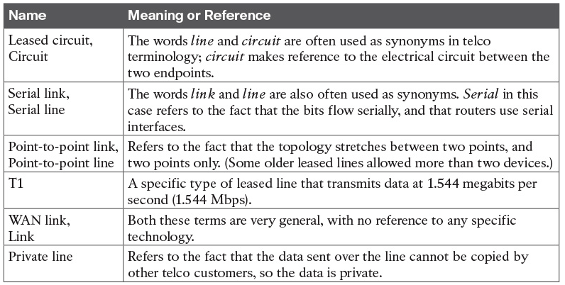
Different Names for a Leased Line
Leased-Line Cabling
To create a leased line, some physical path must exist between the two routers on the ends of the link.
The physical cabling must leave the buildings where each router sits.
However, the telco does not simply install one cable between the two buildings. Instead, it uses what is typically a large and complex network that creates the appearance of a cable between the two routers.
The diagram below gives a little insight into the cabling that could exist inside the telco for a short leased line.
Telcos put their equipment in buildings called central offices (CO). The telco installs cables from the CO to most every other building in the city, expecting to sell services to the people in those buildings one day.
The telco would then configure its switches to use some of the capacity on each cable to send data in both directions, creating the equivalent of a crossover cable between the two routers.
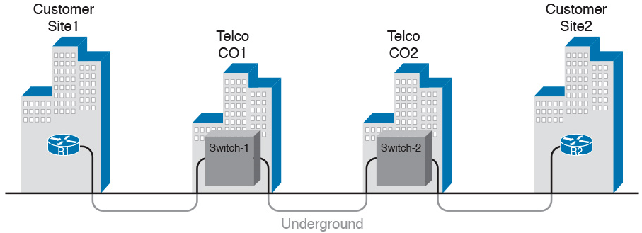
Possible Cabling Inside a Telco for a Short Leased Line
Although what happens inside the telco is completely hidden from the telco customer, enterprise engineers do need to know about the parts of the link that exist inside the customer’s building at the router.
First, each site has customer premises equipment (CPE), which includes the router, serial interface card, and CSU/DSU.
Each router uses a serial interface card that acts somewhat like an Ethernet NIC, sending and receiving data over the physical link.
The physical link requires a function called a channel service unit/data service unit (CSU/DSU). The CSU/DSU can either be integrated into the serial interface card in the router or sit outside the router as an external device.
The diagram below shows the CPE devices, along with the cabling.
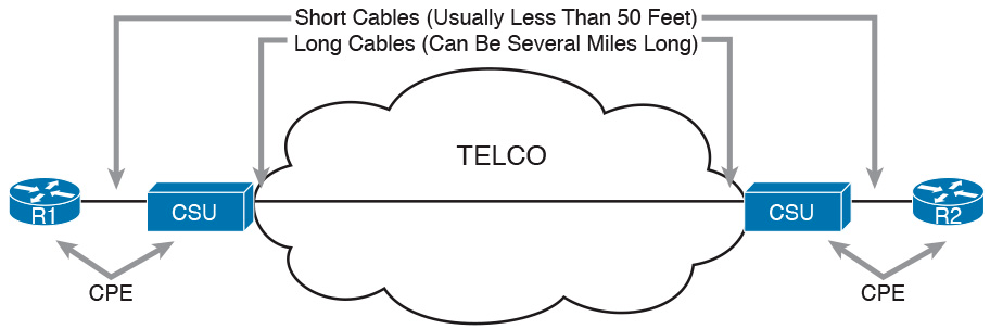
Point-to-Point Leased Line: Components and Terminology
The cabling includes a short serial cable (only if an external CSU/DSU is used) plus the cable installed by the telco for the leased line itself.
The serial cable connects the router serial interface to the external CSU/DSU. (Many cable options exist; the cable just needs to match the connector of the serial interface on one end and the CSU/DSU on the other end.)
The four-wire cable from the telco plugs in to the CSU/DSU, typically using an RJ-48 connector that has the same size and shape as an RJ-45 connector.
Telcos offer a wide variety of speeds for leased lines. However, you cannot pick the exact speed you want; instead, you must pick from a long list of predefined speeds.
Slower-speed links run at multiples of 64 kbps (kilobits per second), while faster links run at multiples of about 1.5 Mbps (megabits per second).
Building a WAN Link in a Lab
One can create the equivalent of a leased line without a real leased line from a telco, and without CSU/DSUs, just using a cabling trick.
First, the serial cables normally used between a router and an external CSU/DSU are called data terminal equipment (DTE) cables.
To create a physical WAN link in a lab, you need two serial cables: one serial DTE cable, plus a similar but slightly different matching data communications equipment (DCE) cable.
The DCE cable has a female connector, while the DTE cable has a male connector, which allows the two cables to be attached directly.
The DCE cable also does the equivalent task of an Ethernet crossover cable by swapping the transmit and receive wire pairs, as shown in the diagram below.
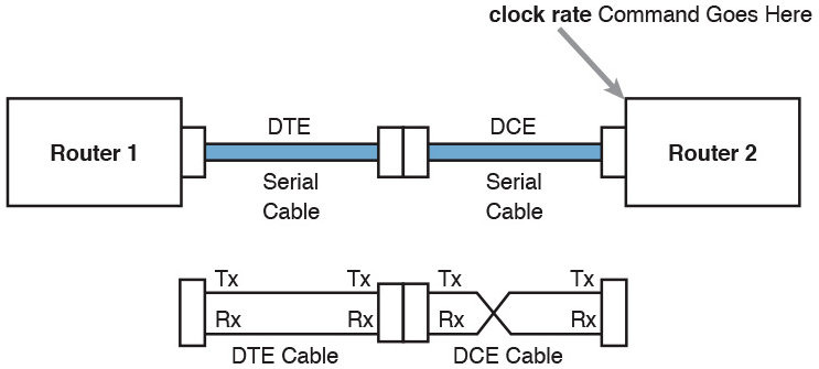
Serial Cabling Uses a DTE Cable and a DCE Cable
The diagram shows the cable details at the top, with the wiring details inside the cable at the bottom.
In particular, at the bottom of the figure, note that the DCE cable swaps the transmit and receive pairs, whereas the DTE serial cable does not, acting as a straight-through cable.
Finally, to make the link work, the router with the DCE cable installed must do one function normally done by the CSU/DSU. The CSU/DSU normally provides a function called clocking, in which it tells the router exactly when to send each bit through signaling over the serial cable.
A router serial interface can provide clocking, and the more recent router software versions automatically supply clocking when the router senses a DCE cable is plugged into the serial port.
Regardless of whether a router has an older or newer software version, you will want to know how to configure serial clocking using the clock rate command
Data-Link Details of Leased Lines
A leased line provides a Layer 1 service.
In other words, it promises to deliver bits between the devices connected to the leased line.
However, the leased line itself does not define a data link layer protocol to be used on the leased line.Because leased lines define only the Layer 1 transmission service, many companies and standards organizations have created data-link protocols to control and use leased lines.
Today, the two most popular data link layer protocols used for leased lines between two routers are High-Level Data Link Control (HDLC) and Point-to-Point Protocol (PPP).
HDLC Basics
All data-link protocols perform a similar role: to control the correct delivery of data over a physical link of a particular type.
For example, the Ethernet data-link protocol uses a destination address field to identify the correct device that should receive the data, and an FCS field that allows the receiving device to determine whether the data arrived correctly. HDLC provides similar functions.
HDLC has less work to do because of the simple point-to-point topology of a point-to-point leased line.
When one router sends an HDLC frame, it can go only one place: to the other end of the link.
So, while HDLC has an address field, the destination is implied.
HDLC has other fields and functions similar to Ethernet as well.
The table below lists the HDLC fields, with the similar Ethernet header/trailer field.
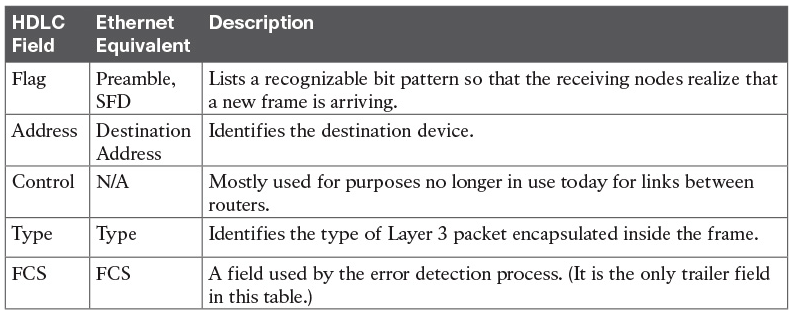
Comparing HDLC Header Fields to Ethernet
HDLC exists today as a standard of the International Organization for Standardization (ISO), the same organization that brought us the OSI model.
However, ISO standard HDLC does not have a Type field, and routers need to know the type of packet inside the frame. So, Cisco routers use a Cisco-proprietary variation of HDLC that adds a Type field, as shown in the diagram below.
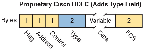
HDLC Framing
How Routers Use a WAN Data Link
Today, most leased lines connect to routers, and routers focus on delivering packets to a destination host.
However, routers physically connect to both LANs and WANs, with those LANs and WANs requiring that data be sent inside data-link frames.
So, now that you know a little about HDLC, it helps to think about how routers use the HDLC protocol when sending data.
First, the TCP/IP network layer focuses on forwarding IP packets from the sending host to the destination host. The underlying LANs and WANs just act as a way to move the packets to the next router or end-user device. The diagram below shows that network layer perspective.
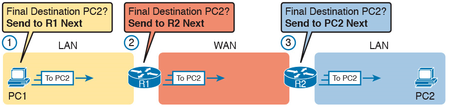
IP Routing Logic over LANs and WANs
Following the steps in the figure, for a packet sent by PC1 to PC2’s IP address:
- PC1’s network layer (IP) logic tells it to send the packet to a nearby router (R1).
- Router R1’s network layer logic tells it to forward (route) the packet out the leased line to Router R2 next.
- Router R2’s network layer logic tells it to forward (route) the packet out the LAN link to PC2 next.
While the diagram above shows the network layer logic, the PCs and routers must rely on the LANs and WANs in the diagram to actually move the bits in the packet.
The diagram below shows the same figure, with the same packet, but this time showing some of the data link layer logic used by the hosts and routers.
Basically, three separate data link layer steps encapsulate the packet, inside a data-link frame, over three hops through the internetwork: from PC1 to R1, from R1 to R2, and from R2 to PC2
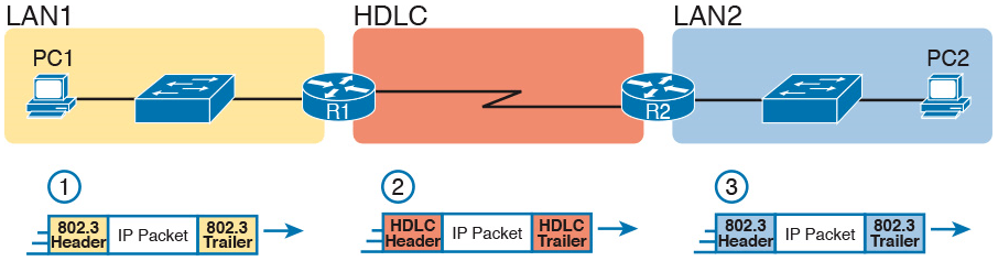
General Concept of Routers De-encapsulating and Re-encapsulating IP Packets
Following the steps in the diagram, again for a packet sent by PC1 to PC2’s IP address:
- To send the IP packet to Router R1 next, PC1 encapsulates the IP packet in an Ethernet frame that has the destination MAC address of R1.
- Router R1 de-encapsulates (removes) the IP packet from the Ethernet frame, encapsulates the packet into an HDLC frame using an HDLC header and trailer, and forwards the HDLC frame to Router R2 next.
- Router R2 de-encapsulates (removes) the IP packet from the HDLC frame, encapsulates the packet into an Ethernet frame that has the destination MAC address of PC2, and forwards the Ethernet frame to PC2.
In summary, a leased line with HDLC creates a WAN link between two routers so that they can forward packets for the devices on the attached LANs.
The leased line itself provides the physical means to transmit the bits, in both directions. The HDLC frames provide the means to encapsulate the network layer packet correctly so that it crosses the link between routers.
Leased lines have many benefits that have led to their relatively long life in the WAN marketplace. These lines are simple for the customer, are widely available, are of high quality, and are private.
However, they do have some negatives as well compared to newer WAN technologies, including a higher cost and typically longer lead times to get the service installed.
Ethernet as a WAN Technology
For the first several decades of the existence of Ethernet, Ethernet was only appropriate for LANs.
The restrictions on cable lengths and devices might allow a LAN that stretched a kilometer or two, to support a campus LAN, but that was the limit.
As time passed, the IEEE improved Ethernet standards in ways that made Ethernet a reasonable WAN technology.
For example, the 1000BASE-LX standard uses single-mode fiber cabling, with support for a 5-km cable length; the 1000BASE-ZX standard supports an even longer 70-km cable length.
As time went by, and as the IEEE improved cabling distances for fiber Ethernet links, Ethernet became a reasonable WAN technology.
Today, in this second decade of the twenty-first century, many WAN service providers (SP) offer WAN services that take advantage of Ethernet.
SPs offer a wide variety of these Ethernet WAN services, with many different names. But all of them use a similar model, with Ethernet used between the customer site and the SP’s network, as shown in the diagram below.
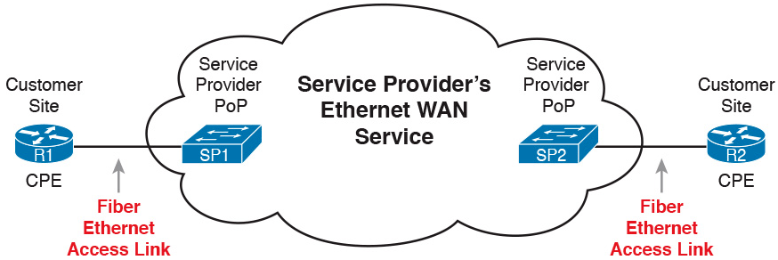
Fiber Ethernet Link to Connect a CPE Router to a Service Provider’s WAN
The customer connects to an Ethernet link using a router interface. The (fiber) Ethernet link leaves the customer building and connects to some nearby SP location called a point of presence (PoP).
Instead of a telco switch, the SP uses an Ethernet switch. Inside the SP’s network, the SP uses any technology that it wants to create the specific Ethernet WAN services.
Ethernet WANs that Create a Layer 2 Service
The WAN services implied by the previous diagram include a broad number of services, with a lot of complex networking concepts needed to understand those services.
The one Ethernet WAN service goes by two names: Ethernet emulation and Ethernet over MPLS (EoMPLS).
Ethernet emulation is a general term, meaning that the service acts like one Ethernet link.
EoMPLS refers to Multiprotocol Label Switching (MPLS), which is one technology that can be used inside the SP’s cloud.
The EoMPLS service provides:
- A point-to-point connection between two customer devices
- Behavior as if a fiber Ethernet link existed between the two devices
So, if you can imagine two routers, with a single Ethernet link between the two routers, you understand what this particular EoMPLS service does.
The diagram below shows the idea. In this case, the two routers, R1 and R2, connect with an EoMPLS service instead of a serial link. The routers use Ethernet interfaces, and they can send data in both directions at the same time. Physically, each router actually connects to some SP PoP, but logically, the two routers can send Ethernet frames to each other over the link.

EoMPLS Acting Like a Simple Ethernet Link Between Two Routers
How Routers Route IP Packets Using Ethernet Emulation
WANs, by their very nature, give IP routers a way to forward IP packets from a LAN at one site, over the WAN, and to another LAN at another site.
Routing over an EoMPLS WAN link still uses the WAN like a WAN, as a way to forward IP packets from one site to another.
However, the WAN link happens to use the same Ethernet protocols as the Ethernet LAN links at each site.
The EoMPLS link uses Ethernet for both Layer 1 and Layer 2 functions. That means the link uses the same familiar Ethernet header and trailer, as shown in the middle the diagram below.
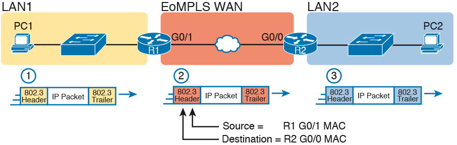
Routing over an EoMPLS Link
All three routing steps use the same Ethernet (802.3) protocol. However, note that each frame’s data-link header and trailer are different.
Each router discards the old data-link header/trailer and adds a new set, as described in these steps.
- To send the IP packet to Router R1 next, PC1 encapsulates the IP packet in an Ethernet frame that has the destination MAC address of R1.
- Router R1 de-encapsulates (removes) the IP packet from the Ethernet frame and encapsulates the packet into a new Ethernet frame, with a new Ethernet header and trailer. The destination MAC address is R2’s G0/0 MAC address, and the source MAC address is R1’s G0/1 MAC address. R1 forwards this frame over the EoMPLS service to R2 next.
- Router R2 de-encapsulates (removes) the IP packet from the Ethernet frame, encapsulates the packet into an Ethernet frame that has the destination MAC address of PC2, and forwards the Ethernet frame to PC2.
Accessing the Internet
Two other popular WAN technologies used to gain access to the Internet: digital subscriber line (DSL) and cable.
These two WAN technologies do not replace leased lines in all cases, but they do play an important role in the specific case of creating a WAN connection between a home or office and the Internet.
The Internet as a Large WAN
The Internet is an amazing cultural phenomenon. Most of us use it every day. We post messages on social media sites, we search for information using a search engine like Google, and we send emails.
We use apps on our phones to pull down information, like weather reports, maps, and movie reviews.
We use the Internet to purchase physical products and to buy and download digital products like music and videos. The Internet has created completely new things to do and changed the old ways of living life compared to a generation ago.
However, if you instead focus on the networking technology that creates the Internet, the Internet is simply one huge TCP/IP network.
In fact, the name “Internet” comes from the core network layer protocol: Internet Protocol. The Internet includes many LANs, and because the Internet spans the globe, it of course needs WAN links to connect different sites.
As a network of networks, the Internet is actually owned by countless companies and people.
The Internet includes most every enterprise TCP/IP network and a huge number of home-based networks, as well as a huge number of individuals from their phones and other wireless devices, as shown in the diagram below.
Internet with Enterprise, Home, and Phone Subscribers
The middle of the Internet, called the Internet core, exists as LANs and WANs owned and operated by Internet service providers (ISP).
(The diagram above shows the Internet core as a cloud, because network diagrams show a cloud when hiding the details of a part of the network.)
ISPs cooperate to create a mesh of links between each other in the Internet core, so that no matter through which ISP a particular company or person connects, some path exists to every device.
The diagram below shows a slightly different version, in this case showing the concept of the Internet core: ISP networks that connect to both their customers as well as each other, so that IP packets can flow from every customer of every ISP to every other customer of every other ISP.
Internet Core with Multiple ISPs and Telcos
Internet Access (WAN) Links
The Internet also happens to use a huge number of WAN links.
All of those lines connecting an enterprise or home to one of the ISPs in above diagram represent some kind of WAN link that uses a cable, while the phones create their WAN link using wireless technology.
These links usually go by the name Internet access link.
Historically, businesses tend to use one set of WAN technologies as Internet access links, while home-based consumers use others.
Businesses often use leased lines, connecting a router at the business to a router at the ISP. The top of the diagram below shows just such an example.
Three Examples of Internet Access Links
Consumers often use technologies like DSL and cable for Internet access links.
These technologies use cabling that is already installed in most homes, making these services somewhat inexpensive for home users.
DSL uses the analog phone lines that are already installed in homes, while cable Internet uses the cable TV (CATV) cable.
While DSL and cable are popular with consumers, many businesses use these technologies for Internet access.
All three of the Internet access technologies in the diagram above happen to use a pair of routers: one at the customer side of the WAN link and one at the ISP side.
The routers will continue to think about network layer logic, of sending IP packets to their destination by forwarding the packets to the next router.
However, the physical and data link layer details on the WAN link differ as compared to leased lines.
Digital Subscriber Line
Digital subscriber line (DSL) creates a relatively short (miles long, not tens of miles) high-speed link WAN between a telco customer and an ISP.
To do so, it uses the same single-pair telephone line used for a typical home phone line.
DSL, as a technology, does not try to replace leased lines, which run between any two sites, for potentially very long distances.
DSL instead just provides a short physical link from a home to the telco’s network, allowing access to the Internet.
First, to get an idea about the cabling, think of a typical home. Each home has one phone line that runs from a nearby telco CO to the home.
As shown on the left side of diagram below, the telephone wiring splits out and terminates at several wall plates, often with RJ-11 ports that are a slightly skinnier cousin of the RJ-45 connector.

Typical Voice Cabling Concepts in the United States
Next, think about the telephone line and the equipment at the CO.
Sometime in the past, the telco installed all the telephone lines from its local CO to each neighborhood, apartment, and so on.
At the CO, each line connects to a port on a telco switch. This switch supports the ability to set up voice calls, take them down, and forward the voice through the worldwide voice network, called the public switched telephone network, or PSTN.
To add DSL service at the home int the above diagram, two changes need to be made.
First, you need to add DSL-capable devices at the home.
Second, the telco has to add DSL equipment at the CO.
Together, the DSL equipment at each side of the local telephone line can send data while still supporting the same voice traffic.
The left side of below diagram shows the changes.

Wiring and Devices for a Home DSL Link
A new DSL modem now connects to a spare phone outlet.
The DSL modem follows the DSL physical and data link layer standards to send data to/from the telco.
The home now has a small LAN, implemented with a consumer-grade router, which often includes an Ethernet switch and possibly a wireless LAN access point.
(Note that the telephones may now also need a short extra cable with a filter in it, installed at the wall jack, to filter out the sounds of the higher electrical frequencies used for DSL.)
The home-based router on the left must be able to send data to/from the Internet.
To make that happen, the telco CO uses a product called a DSL access multiplexer (DSLAM).
The DSLAM splits out the data over to the router on the lower right, which completes the connection to the Internet. The DSLAM also splits out the voice signals over to the voice switch on the upper right.
DSL gives telcos a useful high-speed Internet service to offer their customers.
Telcos have had other offerings that happen to use the same telephone line for data, but these options ran much slower than DSL.
DSL supports asymmetric speeds, meaning that the transmission speed from the ISP toward the home (downstream) is much faster than the transmissions toward the ISP (upstream).
Asymmetric speeds work better for consumer Internet access from the home, because clicking a web page sends only a few hundred bytes upstream into the Internet, but can trigger many megabytes of data to be delivered downstream to the home.
Cable Internet
Cable Internet creates an Internet access service which, when viewed generally rather than specifically, has many similarities to DSL.
Like DSL, cable Internet takes full advantage of existing cabling, using the existing cable TV (CATV) cable to send data.
Like DSL, cable Internet uses asymmetric speeds, sending data faster downstream than upstream, which works better than symmetric speeds for most consumer locations.
And like DSL, cable Internet does not attempt to replace long leased lines between any two sites, instead focusing on the short WAN links from a customer to an ISP.
Cable Internet also uses the same basic in-home cabling concepts as does DSL.
The diagram below shows a diagram similar to DSL, but with the DSL details replaced with cable Internet details.
The telephone line has been replaced with coaxial cable from the CATV company, and the DSL modem has been replaced by a cable modem.
Otherwise, the details in the home follow the same overall plan.
Wiring and Devices for a Home Cable Internet Link
On the CATV company side of the cable Internet service, the CATV company has to split out the data and video, as shown on the right side of the diagram.
Data flows to the lower right, through a router, while video comes in from video dishes for distribution out to the TVs in people’s homes.
Cable Internet service and DSL directly compete for consumer and small-business Internet access.
Generally speaking, while both offer high speeds, cable Internet typically runs at faster speeds than DSL, with DSL providers keeping their prices a little lower to compete.
Both support asymmetric speeds, and both provide an “always on” service, in that you can communicate with the Internet without the need to first take some action to start the Internet connection.

Fundamentals of TCP/IP Networking – Detailed Discussion
INTERNOLD NETWORKS CCNA LIVE WEBCLASS (INCLW)
Fundamentals of TCP/IP Networking
Contents
Introduction to TCP/IP Networking
Let's start with the basics of networking.
Because networks require all the devices to follow the rules, this part starts with a discussion of networking models, which gives you a big-picture view of the networking rules.
You can think of a networking model as you think of a set of architectural plans for building a house. A lot of different people work on building your house, such as framers, electricians, bricklayers, painters, and so on.
The blueprint helps ensure that all the different pieces of the house work together as a whole.
Similarly, the people who make networking products, and the people who use those products to build their own computer networks, follow a particular networking model.
That networking model defines rules about how each part of the network should work, as well as how the parts should work together, so that the entire network functions correctly.
Transmission Control Protocol/Internet Protocol (TCP/IP). TCP/IP is the most pervasively used networking model in the history of networking.
You can find support for TCP/IP on practically every computer operating system (OS) in existence today, from mobile phones to mainframe computers.
Every network built using Cisco products today supports TCP/IP.
TCP/IP is compared to a second networking model, called the Open Systems Interconnection (OSI) reference model.
Historically, OSI was the first large effort to create a vendor-neutral networking model. Because of that timing, many of the terms used in networking today come from the OSI model.
Perspectives on Networking
So, you are new to networking. Like many people, your perspective about networks might be that of a user of the network, as opposed to the network engineer who builds networks.
For some, your view of networking might be based on how you use the Internet, from home, using a high-speed Internet connection like digital subscriber line (DSL) or cable TV, as shown in the diagram below.

End-User Perspective on High-Speed Internet Connections
The top part of the figure shows a typical high-speed cable Internet user.
The PC connects to a cable modem using an Ethernet cable. The cable modem then connects to a cable TV (CATV) outlet in the wall using a round coaxial cable—the same kind of cable used to connect your TV to the CATV wall outlet.
Because cable Internet services provide service continuously, the user can just sit down at the PC and start sending email, browsing websites, making Internet phone calls, and using other tools and applications.
The lower part of the figure uses two different technologies.
First, the tablet computer uses wireless technology that goes by the name wireless local-area network (wireless LAN), or Wi-Fi, instead of using an Ethernet cable. In this example, the router uses a different technology, DSL, to communicate with the Internet.
Both home-based networks and networks built for use by a company make use of similar networking technologies. The Information Technology (IT) world refers to a network created by one corporation, or enterprise, for the purpose of allowing its employees to communicate, as an enterprise network.
The smaller networks at home, when used for business purposes, often go by the name small office/home office (SOHO) networks.
Users of enterprise networks have some idea about the enterprise network at their company or school. People realize that they use a network for many tasks.
PC users might realize that their PC connects through an Ethernet cable to a matching wall outlet, as shown at the top of diagram below. Those same users might use wireless LANs with their laptop when going to a meeting in the conference room as well. The diagram shows these two end-user perspectives on an enterprise network.

Example Representation of an Enterprise Network
NOTE: In networking diagrams, a cloud represents a part of a network whose details are not important to the purpose of the diagram. In this case, the above diagram ignores the details of how to create an enterprise network.
Some users might not even have a concept of the network at all.
Instead, these users just enjoy the functions of the network—the ability to post messages to social media sites, make phone calls, search for information on the Internet, listen to music, and download countless apps to their phones—without caring about how it works or how their favorite device connects to the network.
In the building business, much work happens before you nail the first boards together. The process starts with some planning, an understanding of how to build a house, and some architectural blueprints of how to build that specific house.
Similarly, the journey toward building any computer network does not begin by installing devices and cables, but instead by looking at the architectural plans for those modern networks: the TCP/IP model.
TCP/IP Networking Model
A networking model, sometimes also called either a networking architecture or networking blueprint, refers to a comprehensive set of documents.
Individually, each document describes one small function required for a network; collectively, these documents define everything that should happen for a computer network to work.
Some documents define a protocol, which is a set of logical rules that devices must follow to communicate.
Other documents define some physical requirements for networking. For example, a document could define the voltage and current levels used on a particular cable when transmitting data.
You can think of a networking model as you think of an architectural blueprint for building a house.
Sure, you can build a house without the blueprint.
However, the blueprint can ensure that the house has the right foundation and structure so that it will not fall down, and it has the correct hidden spaces to accommodate the plumbing, electrical, gas, and so on.
Also, the many different people that build the house using the blueprint—such as framers, electricians, bricklayers, painters, and so on—know that if they follow the blueprint, their part of the work should not cause problems for the other workers.
Similarly, you could build your own network—write your own software, build your own networking cards, and so on—to create a network.
However, it is much easier to simply buy and use products that already conform to some well-known networking model or blueprint.
Because the networking product vendors build their products with some networking model in mind, their products should work well together.
History Leading to TCP/IP
Today, the world of computer networking uses one networking model: TCP/IP.
However, the world has not always been so simple.
Once upon a time, networking protocols didn’t exist, including TCP/IP.
Vendors created the first networking protocols; these protocols supported only that vendor’s computers.
For example, IBM published its Systems Network Architecture (SNA) networking model in 1974.
Other vendors also created their own proprietary networking models.
As a result, if your company bought computers from three vendors, network engineers often had to create three different networks based on the networking models created by each company, and then somehow connect those networks, making the combined networks much more complex.
The left side of the diagram below shows the general idea of what a company’s enterprise network might have looked like back in the 1980s, before TCP/IP became common in enterprise internetworks.

Historical Progression: Proprietary Models to the Open TCP/IP Model
Although vendor-defined proprietary networking models often worked well, having an open, vendor-neutral networking model would aid competition and reduce complexity.
The International Organization for Standardization (ISO) took on the task to create such a model, starting as early as the late 1970s, beginning work on what would become known as the Open Systems Interconnection (OSI) networking model.
ISO had a noble goal for the OSI model: to standardize data networking protocols to allow communication among all computers across the entire planet.
ISO worked toward this ambitious and noble goal, with participants from most of the technologically developed nations on Earth participating in the process.
A second, less-formal effort to create an open, vendor-neutral, public networking model sprouted forth from a U.S. Department of Defense (DoD) contract.
Researchers at various universities volunteered to help further develop the protocols surrounding the original DoD work. These efforts resulted in a competing open networking model called TCP/IP.
During the 1990s, companies began adding OSI, TCP/IP, or both to their enterprise networks. However, by the end of the 1990s, TCP/IP had become the common choice, and OSI fell away.
The center part of diagram above shows the general idea behind enterprise networks in that decade—still with networks built upon multiple networking models but including TCP/IP.
Here in the twenty-first century, TCP/IP dominates.
Proprietary networking models still exist, but they have mostly been discarded in favor of TCP/IP.
The OSI model, whose development suffered in part because of a slower formal standardization process as compared with TCP/IP, never succeeded in the marketplace.
And TCP/IP, the networking model originally created almost entirely by a bunch of volunteers, has become the most prolific network model ever, as shown on the right side of diagram above.
Overview of the TCP/IP Networking Model
The TCP/IP model both defines and references a large collection of protocols that allow computers to communicate.
To define a protocol, TCP/IP uses documents called Requests For Comments (RFC). (You can find these RFCs using any online search engine.)
The TCP/IP model also avoids repeating work already done by some other standards body or vendor consortium by simply referring to standards or protocols created by those groups.
For example, the Institute of Electrical and Electronic Engineers (IEEE) defines Ethernet LANs; the TCP/IP model does not define Ethernet in RFCs, but refers to IEEE Ethernet as an option.
An easy comparison can be made between telephones and computers that use TCP/IP. You go to the store and buy a phone from one of a dozen different vendors.
When you get home and plug in the phone to the same cable in which your old phone was connected, the new phone works.
The phone vendors know the standards for phones in their country and build their phones to match those standards.
Similarly, when you buy a new computer today, it implements the TCP/IP model to the point that you can usually take the computer out of the box, plug in all the right cables, turn it on, and it connects to the network. You can use a web browser to connect to your favorite website.
How?
Well, the OS on the computer implements parts of the TCP/IP model.
The Ethernet card, or wireless LAN card, built in to the computer implements some LAN standards referenced by the TCP/IP model.
In short, the vendors that created the hardware and software implemented TCP/IP.
To help people understand a networking model, each model breaks the functions into a small number of categories called layers.
Each layer includes protocols and standards that relate to that category of functions. TCP/IP actually has two alternative models, as shown in the diagram below.

Two TCP/IP Networking Models
The model on the left shows the original TCP/IP model listed in RFC 1122, which breaks TCP/IP into four layers.
The top two layers focus more on the applications that need to send and receive data.
The bottom layer focuses on how to transmit bits over each individual link, with the Internet layer focusing on delivering data over the entire path from the original sending computer to the final destination computer.
The TCP/IP model on the right shows the more common terms and layers used when people talk about TCP/IP today.
It expands the original model’s link layer into two separate layers: data link and physical (similar to the lower two layers of the OSI model). Also, many people commonly use the word “Network” instead of “Internet” for one layer.
NOTE: The original TCP/IP model’s link layer has also been referred to as the network access and network interface layer.
Many of you will have already heard of several TCP/IP protocols, like the examples listed in the table below.

TCP/IP Architectural Model and Example Protocols
TCP/IP Application Layer
TCP/IP application layer protocols provide services to the application software running on a computer.
The application layer does not define the application itself, but it defines services that applications need.
For example, application protocol HTTP defines how web browsers can pull the contents of a web page from a web server. In short, the application layer provides an interface between software running on a computer and the network itself.
Arguably, the most popular TCP/IP application today is the web browser. Many major software vendors either have already changed or are changing their application software to support access from a web browser.
And thankfully, using a web browser is easy: You start a web browser on your computer and select a website by typing the name of the website, and the web page appears.
HTTP Overview
What really happens to allow that web page to appear on your web browser?
Imagine that Bob opens his browser. His browser has been configured to automatically ask for web server Larry’s default web page, or home page. The general logic looks like the diagram below.

Basic Application Logic to Get a Web Page
So, what really happened?
Bob’s initial request actually asks Larry to send his home page back to Bob.
Larry’s web server software has been configured to know that the default web page is contained in a file called home.htm.
Bob receives the file from Larry and displays the contents of the file in Bob’s web browser window.
HTTP Protocol Mechanisms
Taking a closer look, this example shows how applications on each endpoint computer—specifically, the web browser application and web server application—use a TCP/IP application layer protocol.
To make the request for a web page and return the contents of the web page, the applications use the Hypertext Transfer Protocol (HTTP).
HTTP did not exist until Tim Berners-Lee created the first web browser and web server in the early 1990s.
Berners-Lee gave HTTP functionality to ask for the contents of web pages, specifically by giving the web browser the ability to request files from the server and giving the server a way to return the content of those files.
The overall logic matches what was shown in above diagram.
Diagram below shows the same idea, but with details specific to HTTP.

HTTP GET Request, HTTP Reply, and One Data-Only Message
NOTE: The full version of most web addresses—also called Uniform Resource Locators (URL) or Universal Resource Identifiers (URI)—begins with the letters http, which means that HTTP is used to transfer the web pages.
To get the web page from Larry, at Step 1, Bob sends a message with an HTTP header.
Generally, protocols use headers as a place to put information used by that protocol. This HTTP header includes the request to “get” a file.
The request typically contains the name of the file (home.htm, in this case), or if no filename is mentioned, the web server assumes that Bob wants the default web page.
Step 2 in the diagram above shows the response from web server Larry. The message begins with an HTTP header, with a return code (200), which means something as simple as “OK” returned in the header.
HTTP also defines other return codes so that the server can tell the browser whether the request worked.
(Here is another example: If you ever looked for a web page that was not found, and then received an HTTP 404 “not found” error, you received an HTTP return code of 404.)
The second message also includes the first part of the requested file.
Step 3 in the diagram shows another message from web server Larry to web browser Bob, but this time without an HTTP header.
HTTP transfers the data by sending multiple messages, each with a part of the file. Rather than wasting space by sending repeated HTTP headers that list the same information, these additional messages simply omit the header.
TCP/IP Transport Layer
Although many TCP/IP application layer protocols exist, the TCP/IP transport layer includes a smaller number of protocols.
The two most commonly used transport layer protocols are the Transmission Control Protocol (TCP) and the User Datagram Protocol (UDP).
Transport layer protocols provide services to the application layer protocols that reside one layer higher in the TCP/IP model.
How does a transport layer protocol provide a service to a higher-layer protocol?
TCP Error Recovery Basics
To appreciate what the transport layer protocols do, you must think about the layer above the transport layer, the application layer.
Why?
Well, each layer provides a service to the layer above it, like the error-recovery service provided to application layer protocols by TCP.
For example, in the previous diagram, Bob and Larry used HTTP to transfer the home page from web server Larry to Bob’s web browser.
But what would have happened if Bob’s HTTP GET request had been lost in transit through the TCP/IP network?
Or, what would have happened if Larry’s response, which included the contents of the home page, had been lost?
Well, as you might expect, in either case, the page would not have shown up in Bob’s browser.
TCP/IP needs a mechanism to guarantee delivery of data across a network. Because many application layer protocols probably want a way to guarantee delivery of data across a network, the creators of TCP included an error-recovery feature.
To recover from errors, TCP uses the concept of acknowledgments.
The diagram below outlines the basic idea behind how TCP notices lost data and asks the sender to try again.

TCP Error-Recovery Services as Provided to HTTP
Diagram above shows web server Larry sending a web page to web browser Bob, using three separate messages.
The TCP header shows a sequence number (SEQ) with each message.
In this example, the network has a problem, and the network fails to deliver the TCP message (called a segment) with sequence number 2.
When Bob receives messages with sequence numbers 1 and 3, but does not receive a message with sequence number 2, Bob realizes that message 2 was lost.
That realization by Bob’s TCP logic causes Bob to send a TCP segment back to Larry, asking Larry to send message 2 again.
Same-Layer and Adjacent-Layer Interactions
The example in above diagram also demonstrates a function called adjacent-layer interaction, which refers to the concepts of how adjacent layers in a networking model, on the same computer, work together.
In this example, the higher-layer protocol (HTTP) wants error recovery, and the higher layer uses the next lower-layer protocol (TCP) to perform the service of error recovery; the lower layer provides a service to the layer above it.
The diagram also shows an example of a similar function called same-layer interaction.
When a particular layer on one computer wants to communicate with the same layer on another computer, the two computers use headers to hold the information that they want to communicate.
For example, Larry set the sequence numbers to 1, 2, and 3 so that Bob could notice when some of the data did not arrive.
Larry’s TCP process created that TCP header with the sequence number; Bob’s TCP process received and reacted to the TCP segments.
The table below summarizes the key points about how adjacent layers work together on a single computer and how one layer on one computer works with the same networking layer on another computer.

Summary: Same-Layer and Adjacent-Layer Interactions
TCP/IP Network Layer
The application layer includes many protocols. The transport layer includes fewer protocols, most notably, TCP and UDP.
The TCP/IP network layer includes a small number of protocols, but only one major protocol: the Internet Protocol (IP).
In fact, the name TCP/IP is simply the names of the two most common protocols (TCP and IP) separated by a /.
IP provides several features, most importantly, addressing and routing.
Internet Protocol and the Postal Service
Imagine that you just wrote two letters: one to a friend on the other side of the country and one to a friend on the other side of town.
You addressed the envelopes and put on the stamps, so both are ready to give to the postal service. Is there much difference in how you treat each letter?
Not really.
Typically, you would just put them in the same mailbox and expect the postal service to deliver both letters.
The postal service, however, must think about each letter separately, and then make a decision of where to send each letter so that it is delivered.
For the letter sent across town, the people in the local post office probably just need to put the letter on another truck.
For the letter that needs to go across the country, the postal service sends the letter to another post office, then another, and so on, until the letter gets delivered across the country. At each post office, the postal service must process the letter and choose where to send it next.
To make it all work, the postal service has regular routes for small trucks, large trucks, planes, boats, and so on, to move letters between postal service sites.
The service must be able to receive and forward the letters, and it must make good decisions about where to send each letter next, as shown in the diagram below.

Postal Service Forwarding (Routing) Letters
Still thinking about the postal service, consider the difference between the person sending the letter and the work that the postal service does.
The person sending the letters expects that the postal service will deliver the letter most of the time. However, the person sending the letter does not need to know the details of exactly what path the letters take.
In contrast, the postal service does not create the letter, but it accepts the letter from the customer. Then, the postal service must know the details about addresses and postal codes that group addresses into larger groups, and it must have the ability to deliver the letters.
The TCP/IP application and transport layers act like the person sending letters through the postal service.
These upper layers work the same way regardless of whether the endpoint host computers are on the same LAN or are separated by the entire Internet.
To send a message, these upper layers ask the layer below them, the network layer, to deliver the message.
The lower layers of the TCP/IP model act more like the postal service to deliver those messages to the correct destinations.
To do so, these lower layers must understand the underlying physical network because they must choose how to best deliver the data from one host to another.
So, what does this all matter to networking?
Well, the network layer of the TCP/IP networking model, primarily defined by the Internet Protocol (IP), works much like the postal service.
IP defines that each host computer should have a different IP address, just as the postal service defines addressing that allows unique addresses for each house, apartment, and business.
Similarly, IP defines the process of routing so that devices called routers can work like the post office, forwarding packets of data so that they are delivered to the correct destinations.
Just as the postal service created the necessary infrastructure to deliver letters—post offices, sorting machines, trucks, planes, and personnel—the network layer defines the details of how a network infrastructure should be created so that the network can deliver data to all computers in the network.
NOTE: TCP/IP defines two versions of IP: IP version 4 (IPv4) and IP version 6 (IPv6). The world still mostly uses IPv4
Internet Protocol Addressing Basics
IP defines addresses for several important reasons.
First, each device that uses TCP/IP—each TCP/IP host—needs a unique address so that it can be identified in the network.
IP also defines how to group addresses together, just like the postal system groups addresses based on postal codes (or ZIP codes).
To understand the basics, examine the diagram below, which shows the familiar web server Larry and web browser Bob; but now, instead of ignoring the network between these two computers, part of the network infrastructure is included.

Simple TCP/IP Network: Three Routers with IP Addresses Grouped
First, note that the diagram above shows some sample IP addresses. Each IP address has four numbers, separated by periods.
In this case, Larry uses IP address 1.1.1.1, and Bob uses 2.2.2.2. This style of number is called a dotted-decimal notation (DDN).
The diagram also shows three groups of addresses.
In this example, all IP addresses that begin with 1 must be on the upper left, as shown in shorthand in the figure as 1.__.__.__.
All addresses that begin with 2 must be on the right, as shown in shorthand as 2.__.__.__.
Finally, all IP addresses that begin with 3 must be at the bottom of the diagram.
In addition, the diagram introduces icons that represent IP routers.
Routers are networking devices that connect the parts of the TCP/IP network together for the purpose of routing (forwarding) IP packets to the correct destination.
Routers do the equivalent of the work done by each post office site: They receive IP packets on various physical interfaces, make decisions based on the IP address included with the packet, and then physically forward the packet out some other network interface.
IP Routing Basics
The TCP/IP network layer, using the IP protocol, provides a service of forwarding IP packets from one device to another.
Any device with an IP address can connect to the TCP/IP network and send packets. This section shows a basic IP routing example for perspective.
NOTE: The term IP host refers to any device, regardless of size or power, that has an IP address and connects to any TCP/IP network.
The diagram below repeats the familiar case in which web server Larry wants to send part of a web page to Bob, but now with details related to IP.

Basic Routing Example
On the lower left, note that server Larry has the familiar application data, HTTP header, and TCP header ready to send.
In addition, the message now contains an IP header. The IP header includes a source IP address of Larry’s IP address (1.1.1.1) and a destination IP address of Bob’s IP address (2.2.2.2).
Step 1, begins with Larry being ready to send an IP packet.
Larry’s IP process chooses to send the packet to some router—a nearby router on the same LAN—with the expectation that the router will know how to forward the packet.
(This logic is much like you or me sending all our letters by putting them in a nearby mailbox.)
Larry doesn’t need to know anything more about the topology or the other routers.
At Step 2, Router R1 receives the IP packet, and R1’s IP process makes a decision.
R1 looks at the destination address (2.2.2.2), compares that address to its known IP routes, and chooses to forward the packet to Router R2.
This process of forwarding the IP packet is called IP routing (or simply routing).
At Step 3, Router R2 repeats the same kind of logic used by Router R1.
R2’s IP process will compare the packet’s destination IP address (2.2.2.2) to R2’s known IP routes and make a choice to forward the packet to the right, on to Bob.
TCP/IP Link Layer (Data Link Plus Physical)
The TCP/IP model’s original link layer defines the protocols and hardware required to deliver data across some physical network.
The term link refers to the physical connections, or links, between two devices and the protocols used to control those links.
Just like every layer in any networking model, the TCP/IP link layer provides services to the layer above it in the model.
When a host’s or router’s IP process chooses to send an IP packet to another router or host, that host or router then uses link-layer details to send that packet to the next host/router.
Because each layer provides a service to the layer above it, take a moment to think about the IP logic related to above diagram.
In that example, host Larry’s IP logic chooses to send the IP packet to a nearby router (R1), with no mention of the underlying Ethernet.
The Ethernet network, which implements link-layer protocols, must then be used to deliver that packet from host Larry over to router R1.
The diagram below shows four steps of what occurs at the link layer to allow Larry to send the IP packet to R1.

Larry Using Ethernet to Forward an IP Packet to Router R1
NOTE: Above diagram depicts the Ethernet as a series of lines. Networking diagrams often use this convention when drawing Ethernet LANs, in cases where the actual LAN cabling and LAN devices are not important to some discussion, as is the case here. The LAN would have cables and devices, like LAN switches, which are not shown.
The diagram shows four steps.
The first two occur on Larry, and the last two occur on Router R1, as follows:
- Step 1. Larry encapsulates the IP packet between an Ethernet header and Ethernet trailer, creating an Ethernet frame.
- Step 2. Larry physically transmits the bits of this Ethernet frame, using electricity flowing over the Ethernet cabling.
- Step 3. Router R1 physically receives the electrical signal over a cable, and re-creates the same bits by interpreting the meaning of the electrical signals.
- Step 4. Router R1 de-encapsulates the IP packet from the Ethernet frame by removing and discarding the Ethernet header and trailer.
By the end of this process, the link-layer processes on Larry and R1 have worked together to deliver the packet from Larry to Router R1.
NOTE: Protocols define both headers and trailers for the same general reason, but headers exist at the beginning of the message and trailers exist at the end.
The link layer includes a large number of protocols and standards.
For example, the link layer includes all the variations of Ethernet protocols, along with several other LAN standards that were more popular in decades past.
The link layer includes wide-area network (WAN) standards for different physical media, which differ significantly compared to LAN standards because of the longer distances involved in transmitting the data.
This layer also includes the popular WAN standards that add headers and trailers as shown generally in the diagram—protocols such as the Point-to-Point Protocol (PPP) and Frame Relay.
In short, the TCP/IP link layer includes two distinct functions:
- functions related to the physical transmission of the data
- the protocols and rules that control the use of the physical media
The five-layer TCP/IP model simply splits out the link layer into two layers (data link and physical) to match this logic.
TCP/IP Model and Terminology
Comparing the Original and Modern TCP/IP Models
The original TCP/IP model defined a single layer—the link layer—below the Internet layer.
The functions defined in the original link layer can be broken into two major categories:
- functions related directly to the physical transmission of data
- funstions indirectly related to the physical transmission of data
For example, in the four steps shown in the above diagram, Steps 2 and 3 were specific to sending the data, but Steps 1 and 4—encapsulation and de-encapsulation—were only indirectly related.
Today, most documents use a more modern version of the TCP/IP model, as shown in below.

Link Versus Data Link and Physical Layers
Comparing the two, the upper layers are identical, except a name change from Internet to Network.
The lower layers differ in that the single link layer in the original model is split into two layers to match the division of physical transmission details from the other functions.
Data Encapsulation Terminology
As you can see from the explanations of how HTTP, TCP, IP, and Ethernet do their jobs, each layer adds its own header (and for data-link protocols, also a trailer) to the data supplied by the higher layer.
The term encapsulation refers to the process of putting headers (and sometimes trailers) around some data.
The process by which a TCP/IP host sends data can be viewed as a five-step process.
The first four steps relate to the encapsulation performed by the four TCP/IP layers, and the last step is the actual physical transmission of the data by the host.
In fact, if you use the five-layer TCP/IP model, one step corresponds to the role of each layer.
The steps are summarized in the following list:
- Step 1. Create and encapsulate the application data with any required application layer headers. For example, the HTTP OK message can be returned in an HTTP header, followed by part of the contents of a web page.
- Step 2. Encapsulate the data supplied by the application layer inside a transport layer header. For end-user applications, a TCP or UDP header is typically used.
- Step 3. Encapsulate the data supplied by the transport layer inside a network layer (IP) header. IP defines the IP addresses that uniquely identify each computer.
- Step 4. Encapsulate the data supplied by the network layer inside a data link layer header and trailer. This layer uses both a header and a trailer.
- Step 5. Transmit the bits. The physical layer encodes a signal onto the medium to transmit the frame.
The numbers in the diagram below correspond to the five steps in this list, graphically showing the same concepts. Note that because the application layer often does not need to add a header, the figure does not show a specific application layer header.

Five Steps of Data Encapsulation: TCP/IP
Names of TCP/IP Messages
Finally, take particular care to remember the terms segment, packet, and frame and the meaning of each.
Each term refers to the headers (and possibly trailers) defined by a particular layer and the data encapsulated following that header.
Each term, however, refers to a different layer: segment for the transport layer, packet for the network layer, and frame for the link layer.
The diagram below shows each layer along with the associated term.

Perspectives on Encapsulation and “Data”
The letters LH and LT stand for link header and link trailer, respectively, and refer to the data link layer header and trailer.
The diagram also shows the encapsulated data as simply “data.”
When focusing on the work done by a particular layer, the encapsulated data typically is unimportant.
For example, an IP packet can indeed have a TCP header after the IP header, an HTTP header after the TCP header, and data for a web page after the HTTP header.
However, when discussing IP, you probably just care about the IP header, so everything after the IP header is just called data.
So, when drawing IP packets, everything after the IP header is typically shown simply as data.
OSI Networking Model
At one point in the history of the OSI model, many people thought that OSI would win the battle of the networking models discussed earlier.
If that had occurred, instead of running TCP/IP on every computer in the world, those computers would be running with OSI.
However, OSI did not win that battle.
In fact, OSI no longer exists as a networking model that could be used instead of TCP/IP, although some of the original protocols referenced by the OSI model still exist.
So, why OSI? Terminology.
During those years in which many people thought the OSI model would become commonplace in the world of networking (mostly in the late 1980s and early 1990s), many vendors and protocol documents started using terminology from the OSI model.
That terminology remains today.
So, while you will never need to work with a computer that uses OSI, to understand modern networking terminology, you need to understand something about OSI.
Comparing OSI and TCP/IP
The OSI model has many similarities to the TCP/IP model from a basic conceptual perspective. It has (seven) layers, and each layer defines a set of typical networking functions.
As with TCP/IP, the OSI layers each refer to multiple protocols and standards that implement the functions specified by each layer.
In other cases, just as for TCP/IP, the OSI committees did not create new protocols or standards, but instead referenced other protocols that were already defined.
For example, the IEEE defines Ethernet standards, so the OSI committees did not waste time specifying a new type of Ethernet; it simply referred to the IEEE Ethernet standards.
Today, the OSI model can be used as a standard of comparison to other networking models.
Below diagram compares the seven-layer OSI model with both the four-layer and five-layer TCP/IP models.

OSI Model Compared to the Two TCP/IP Models
Describing Protocols by Referencing the OSI Layers
Even today, networking documents often describe TCP/IP protocols and standards by referencing OSI layers, both by layer number and layer name.
For example, a common description of a LAN switch is “Layer 2 switch,” with “Layer 2” referring to OSI layer 2.
Because OSI did have a well-defined set of functions associated with each of its seven layers, if you know those functions, you can understand what people mean when they refer to a product or function by its OSI layer.
For another example, TCP/IP’s original Internet layer, as implemented mainly by IP, equates most directly to the OSI network layer.
So, most people say that IP is a network layer protocol, or a Layer 3 protocol, using OSI terminology and numbers for the layer.
Of course, if you numbered the TCP/IP model, starting at the bottom, IP would be either Layer 2 or 3, depending on what version of the TCP/IP model you care to use.
However, even though IP is a TCP/IP protocol, everyone uses the OSI model layer names and numbers when describing IP or any other protocol for that matter.
The claim that a particular TCP/IP layer is similar to a particular OSI layer is a general comparison, but not a detailed comparison.
The comparison is a little like comparing a car to a truck: Both can get you from point A to point B, but they have many specific differences, like the truck having a truck bed in which to carry cargo.
Similarly, both the OSI and TCP/IP network layers define logical addressing and routing.
However, the addresses have a different size, and the routing logic even works differently.
So the comparison of OSI layers to other protocol models is a general comparison of major goals, and not a comparison of the specific methods.
OSI Layers and Their Functions
Today, because most people happen to be much more familiar with TCP/IP functions than with OSI functions, one of the best ways to learn about the function of different OSI layers is to think about the functions in the TCP/IP model and to correlate those with the OSI model.
For the purposes of learning, you can think of five of the OSI layers as doing the same kinds of things as the matching five layers in the TCP/IP model.
For example, the application layer of each model defines protocols to be used directly by the applications, and the physical layer of each defines the electro-mechanical details of communicating over physical connections.
Table below briefly describes each OSI layer.

OSI Reference Model Layer Descriptions
While the table below lists a sampling of the devices and protocols and their comparable OSI layers.
Note that many network devices must actually understand the protocols at multiple OSI layers, so the layer listed in the table actually refers to the highest layer that the device normally thinks about when performing its core work.
For example, routers need to think about Layer 3 concepts, but they must also support features at both Layers 1 and 2.

OSI Reference Model: Device and Protocol Examples
Besides remembering the basics of the features of each OSI layer, and some protocol and device example at each layer, you should also memorize the names of the layers.
You can simply memorize them, but some people like to use a mnemonic phrase to make memorization easier.
In the following phrases, the first letter of each word is the same as the first letter of an OSI layer name, in the order specified in parentheses:
- All People Seem To Need Data Processing (Layers 7 to 1)
- Please Do Not Take Sausage Pizzas Away (Layers 1 to 7)
OSI Layering Concepts and Benefits
While networking models use layers to help humans categorize and understand the many functions in a network, networking models use layers for many reasons.
For example, consider another postal service analogy.
A person writing a letter does not have to think about how the postal service will deliver a letter across the country.
The postal worker in the middle of the country does not have to worry about the contents of the letter.
Likewise, networking models that divide functions into different layers enable one software package or hardware device to implement functions from one layer, and assume that other software/hardware will perform the functions defined by the other layers.
The following list summarizes the benefits of layered protocol specifications:
- Less complex: Compared to not using a layered model, network models break the concepts into smaller parts.
- Standard interfaces: The standard interface definitions between each layer allow multiple vendors to create products that fill a particular role, with all the benefits of open competition.
- Easier to learn: Humans can more easily discuss and learn about the many details of a protocol specification.
- Easier to develop: Reduced complexity allows easier program changes and faster product development.
- Multivendor interoperability: Creating products to meet the same networking standards means that computers and networking gear from multiple vendors can work in the same network.
- Modular engineering: One vendor can write software that implements higher layers—for example, a web browser—and another vendor can write software that implements the lower layers—for example, Microsoft’s built-in TCP/IP software in its operating systems.
OSI Encapsulation Terminology
Like TCP/IP, each OSI layer asks for services from the next lower layer.
To provide the services, each layer makes use of a header and possibly a trailer. The lower layer encapsulates the higher layer’s data behind a header.
OSI uses a more generic term to refer to messages, rather than frame, packet, and segment. OSI uses the term protocol data unit (PDU).
A PDU represents the bits that include the headers and trailers for that layer, as well as the encapsulated data.
For example, an IP packet using OSI terminology, is a PDU, more specifically a Layer 3 PDU (abbreviated L3PDU) because IP is a Layer 3 protocol.
OSI simply refers to the Layer x PDU (LxPDU), with x referring to the number of the layer being discussed, as shown in the diagram below.

OSI Encapsulation and Protocol Data Units
Fundamentals of TCP/IP Transport and Applications
TCP/IP Layer 4 Protocols: TCP and UDP
The OSI transport layer (Layer 4) defines several functions, the most important of which are error recovery and flow control.
Likewise, the TCP/IP transport layer protocols also implement these same types of features.
Note that both the OSI model and the TCP/IP model call this layer the transport layer.
But as usual, when referring to the TCP/IP model, the layer name and number are based on OSI, so any TCP/IP transport layer protocols are considered Layer 4 protocols.
The key difference between TCP and UDP is that TCP provides a wide variety of services to applications, whereas UDP does not.
For example, routers discard packets for many reasons, including bit errors, congestion, and instances in which no correct routes are known.
As you have learned already, most data-link protocols notice errors (a process called error detection) but then discard frames that have errors.
TCP provides retransmission (error recovery) and helps to avoid congestion (flow control), whereas UDP does not.
As a result, many application protocols choose to use TCP.
However, do not let UDP’s lack of services make you think that UDP is worse than TCP.
By providing fewer services, UDP needs fewer bytes in its header compared to TCP, resulting in fewer bytes of overhead in the network. UDP software does not slow down data transfer in cases where TCP can purposefully slow down.
Also, some applications, notably today Voice over IP (VoIP) and video over IP, do not need error recovery, so they use UDP.
So, UDP also has an important place in TCP/IP networks today.
Table below lists the main features supported by TCP/UDP. Note that only the first item listed in the table is supported by UDP, whereas all items in the table are supported by TCP.

TCP/IP Transport Layer Features
Transmission Control Protocol
Each TCP/IP application typically chooses to use either TCP or UDP based on the application’s requirements.
For example, TCP provides error recovery, but to do so, it consumes more bandwidth and uses more processing cycles.
UDP does not perform error recovery, but it takes less bandwidth and uses fewer processing cycles.
Regardless of which of these two TCP/IP transport layer protocols the application chooses to use, you should understand the basics of how each of these transport layer protocols works.
TCP, as defined in Request For Comments (RFC) 793, accomplishes the functions listed in table above through mechanisms at the endpoint computers.
TCP relies on IP for end-to-end delivery of the data, including routing issues. In other words, TCP performs only part of the functions necessary to deliver the data between applications.
Also, the role that it plays is directed toward providing services for the applications that sit at the endpoint computers.
Regardless of whether two computers are on the same Ethernet, or are separated by the entire Internet, TCP performs its functions the same way.
The diagram below shows the fields in the TCP header.

TCP Header Fields
The message created by TCP that begins with the TCP header, followed by any application data, is called a TCP segment. Alternatively, the more generic term Layer 4 PDU, or L4PDU, can also be used.
Multiplexing Using TCP Port Numbers
TCP and UDP both use a concept called multiplexing.
Multiplexing by TCP and UDP involves the process of how a computer thinks when receiving data.
The computer might be running many applications, such as a web browser, an email package, or an Internet VoIP application (for example, Skype).
TCP and UDP multiplexing tells the receiving computer to which application to give the received data.
Some examples will help make the need for multiplexing obvious. The sample network consists of two PCs, labeled Hannah and Jessie. Hannah uses an application that she wrote to send advertisements that appear on Jessie’s screen.
The application sends a new ad to Jessie every 10 seconds. Hannah uses a second application, a wire-transfer application, to send Jessie some money.
Finally, Hannah uses a web browser to access the web server that runs on Jessie’s PC.
The ad application and wire-transfer application are imaginary, just for this example.
The web application works just like it would in real life.
The diagram shows the sample network, with Jessie running three applications:
- A UDP-based advertisement application
- A TCP-based wire-transfer application
- A TCP web server application

Hannah Sending Packets to Jessie, with Three Applications
Jessie needs to know which application to give the data to, but all three packets are from the same Ethernet and IP address.
You might think that Jessie could look at whether the packet contains a UDP or TCP header, but as you see in the figure, two applications (wire transfer and web) are using TCP.
TCP and UDP solve this problem by using a port number field in the TCP or UDP header, respectively.
Each of Hannah’s TCP and UDP segments uses a different destination port number so that Jessie knows which application to give the data to.
The diagram below shows an example.

Hannah Sending Packets to Jessie, with Three Applications Using Port Numbers to Multiplex
Multiplexing relies on a concept called a socket. A socket consists of three things:
- An IP address
- A transport protocol
- A port number
So, for a web server application on Jessie, the socket would be (10.1.1.2, TCP, port 80) because, by default, web servers use the well-known port 80.
When Hannah’s web browser connects to the web server, Hannah uses a socket as well—possibly one like this: (10.1.1.1, TCP, 1030).
Why 1030?
Well, Hannah just needs a port number that is unique on Hannah, so Hannah sees that port 1030 is available and uses it.
In fact, hosts typically allocate dynamic port numbers starting at 1024 because the ports below 1024 are reserved for well-known applications.
In diagram above, Hannah and Jessie use three applications at the same time—hence, three socket connections are open.
Because a socket on a single computer should be unique, a connection between two sockets should identify a unique connection between two computers.
This uniqueness means that you can use multiple applications at the same time, talking to applications running on the same or different computers.
Multiplexing, based on sockets, ensures that the data is delivered to the correct applications.
The diagram below shows the three socket connections between Hannah and Jessie.

Connections Between Sockets
Port numbers are a vital part of the socket concept. Well-known port numbers are used by servers; other port numbers are used by clients.
Applications that provide a service, such as FTP, Telnet, and web servers, open a socket using a well-known port and listen for connection requests.
Because these connection requests from clients are required to include both the source and destination port numbers, the port numbers used by the servers must be well-known.
Therefore, each service uses a specific well-known port number.
The well-known ports are listed at www.iana.org/assignments/service-names-port-numbers/service-names-port-numbers.txt.
On client machines, where the requests originate, any locally unused port number can be allocated.
The result is that each client on the same host uses a different port number, but a server uses the same port number for all connections.
For example, 100 web browsers on the same host computer could each connect to a web server, but the web server with 100 clients connected to it would have only one socket and, therefore, only one port number (port 80, in this case).
The server can tell which packets are sent from which of the 100 clients by looking at the source port of received TCP segments.
The server can send data to the correct web client (browser) by sending data to that same port number listed as a destination port.
The combination of source and destination sockets allows all participating hosts to distinguish between the data’s source and destination.
Although the example explains the concept using 100 TCP connections, the same port-numbering concept applies to UDP sessions in the same way.
Popular TCP/IP Applications
Some of the applications that can be used to help manage and control a network are:
- The World Wide Web (WWW) application exists through web browsers accessing the content available on web servers. Although it is often thought of as an end-user application, you can actually use WWW to manage a router or switch. You enable a web server function in the router or switch and use a browser to access the router or switch.
- The Domain Name System (DNS) allows users to use names to refer to computers, with DNS being used to find the corresponding IP addresses. DNS also uses a client/server model, with DNS servers being controlled by networking personnel and DNS client functions being part of most any device that uses TCP/IP today. The client simply asks the DNS server to supply the IP address that corresponds to a given name.
- Simple Network Management Protocol (SNMP) is an application layer protocol used specifically for network device management.
- For example, Cisco supplies a large variety of network management products, many of them in the Cisco Prime network management software product family.
- They can be used to query, compile, store, and display information about a network’s operation. To query the network devices, Cisco Prime software mainly uses SNMP protocols.
- Traditionally, to move files to and from a router or switch, Cisco used Trivial File Transfer Protocol (TFTP). TFTP defines a protocol for basic file transfer—hence the word trivial. Alternatively, routers and switches can use File Transfer Protocol (FTP), which is a much more functional protocol, to transfer files.
- Both work well for moving files into and out of Cisco devices.
- FTP allows many more features, making it a good choice for the general end-user population.
- TFTP client and server applications are very simple, making them good tools as embedded parts of networking devices.
Some of these applications use TCP, and some use UDP.
For example, Simple Mail Transfer Protocol (SMTP) and Post Office Protocol version 3 (POP3), both used for transferring mail, require guaranteed delivery, so they use TCP.
Regardless of which transport layer protocol is used, applications use a well-known port number so that clients know which port to attempt to connect to.
The table below lists several popular applications and their well-known port numbers.

Popular Applications and Their Well-Known Port Numbers
Connection Establishment and Termination
TCP connection establishment occurs before any of the other TCP features can begin their work.
Connection establishment refers to the process of initializing Sequence and Acknowledgment fields and agreeing on the port numbers used.
Diagram below shows an example of connection establishment flow.

TCP Connection Establishment
This three-way connection establishment flow (also called a three-way handshake) must complete before data transfer can begin.
The connection exists between the two sockets, although the TCP header has no single socket field.
Of the three parts of a socket, the IP addresses are implied based on the source and destination IP addresses in the IP header.
TCP is implied because a TCP header is in use, as specified by the protocol field value in the IP header.
Therefore, the only parts of the socket that need to be encoded in the TCP header are the port numbers.
TCP signals connection establishment using 2 bits inside the flag fields of the TCP header.
Called the SYN and ACK flags, these bits have a particularly interesting meaning.
SYN means “synchronize the sequence numbers,” which is one necessary component in initialization for TCP.
Diagram below shows TCP connection termination.
This four-way termination sequence is straightforward and uses an additional flag, called the FIN bit. (FIN is short for “finished,” as you might guess.)
One interesting note: Before the device on the right sends the third TCP segment in the sequence, it notifies the application that the connection is coming down.
It then waits on an acknowledgment from the application before sending the third segment in the figure.
Just in case the application takes some time to reply, the PC on the right sends the second flow in the figure, acknowledging that the other PC wants to take down the connection. Otherwise, the PC on the left might resend the first segment repeatedly.

TCP Connection Termination
TCP establishes and terminates connections between the endpoints, whereas UDP does not.
Many protocols operate under these same concepts, so the terms connection-oriented and connectionless are used to refer to the general idea of each. More formally, these terms can be defined as follows:
- Connection-oriented protocol: A protocol that requires an exchange of messages before data transfer begins, or that has a required pre-established correlation between two endpoints.
- Connectionless protocol: A protocol that does not require an exchange of messages and that does not require a pre-established correlation between two endpoints.
Error Recovery and Reliability
TCP provides for reliable data transfer, which is also called reliability or error recovery.
To accomplish reliability, TCP numbers data bytes using the Sequence and Acknowledgment fields in the TCP header.
TCP achieves reliability in both directions, using the Sequence Number field of one direction combined with the Acknowledgment field in the opposite direction.
Diagram below shows an example of how the TCP sequence and acknowledgment fields allow the PC to send 3000 bytes of data to the server, with the server acknowledging receipt of the data.
The TCP segments in the figure occur in order, from top to bottom.
For simplicity’s sake, all messages happen to have 1000 bytes of data in the data portion of the TCP segment.
The first Sequence number is a nice round number (1000), again for simplicity’s sake.
The top of the figure shows three segments, with each sequence number being 1000 more than the previous, identifying the first of the 1000 bytes in the message. (That is, in this example, the first segment holds bytes 1000–1999; the second holds bytes 2000–2999; and the third holds bytes 3000–3999.)

TCP Acknowledgment Without Errors
The fourth TCP segment in the figure—the only one flowing back from the server to the web browser—acknowledges the receipt of all three segments.
How?
The acknowledgment value of 4000 means “I received all data with sequence numbers up through one less than 4000, so I am ready to receive your byte 4000 next.”
(Note that this convention of acknowledging by listing the next expected byte, rather than the number of the last byte received, is called forward acknowledgment.)
This first example does not recover from any errors, however; it simply shows the basics of how the sending host uses the sequence number field to identify the data, with the receiving host using forward acknowledgments to acknowledge the data.
The more interesting discussion revolves around how to use these same tools to do error recovery.
TCP uses the sequence and acknowledgment fields so that the receiving host can notice lost data, ask the sending host to resend, and then acknowledge that the re-sent data arrived.
Many variations exist for how TCP does error recovery.
Below diagram shows just one such example, with similar details compared to the previous diagram. The web browser again sends three TCP segments, again 1000 bytes each, again with easy-to-remember sequence numbers. However, in this example, the second TCP segment fails to cross the network.

TCP Acknowledgment with Errors
The figure points out three sets of ideas behind how the two hosts think.
First, on the right, the server realizes that it did not receive all the data. The two received TCP segments contain bytes numbered 1000–1999 and 3000–3999.
Clearly, the server did not receive the bytes numbered in between. The server then decides to acknowledge all the data up to the lost data—that is, to send back a segment with the acknowledgment field equal to 2000.
The receipt of an acknowledgment that does not acknowledge all the data sent so far tells the sending host to resend the data.
The PC on the left may wait a few moments to make sure no other acknowledgments arrive (using a timer called the retransmission timer), but will soon decide that the server means “I really do need 2000 next—resend it.” The PC on the left does so, as shown in the fifth of the six TCP segments in the diagram.
Finally, note that the server can acknowledge not only the re-sent data, but any earlier data that had been received correctly.
In this case, the server received the re-sent second TCP segment (the data with sequence numbers 2000–2999), but the server had already received the third TCP segment (the data numbered 3000–3999).
The server’s next acknowledgment field acknowledges the data in both those segments, with an acknowledgment field of 4000.
Flow Control Using Windowing
TCP implements flow control by using a window concept that is applied to the amount of data that can be outstanding and awaiting acknowledgment at any one point in time.
The window concept lets the receiving host tell the sender how much data it can receive right now, giving the receiving host a way to make the sending host slow down or speed up.
The receiver can slide the window size up and down—called a sliding window or dynamic window—to change how much data the sending host can send.
The sliding window mechanism makes much more sense with an example.
The example, shown in diagram below, uses the same basic rules as the examples in the previous few diagrams. In this case, none of the TCP segments have errors, and the discussion begins one TCP segment earlier than in the previous two figures.

TCP Windowing
Begin with the first segment, sent by the server to the PC.
The Acknowledgment field should be familiar by now: it tells the PC that the server expects a segment with sequence number 1000 next.
The new field, the window field, is set to 3000. Because the segment flows to the PC, this value tells the PC that the PC can send no more than 3000 bytes over this connection before receiving an acknowledgment.
So, as shown on the left, the PC realizes it can send only 3000 bytes, and it stops sending, waiting on an acknowledgment, after sending three 1000-byte TCP segments.
Continuing the example, the server not only acknowledges receiving the data (without any loss), but the server decides to slide the window size a little higher.
Note that second message flowing right-to-left in the figure, this time with a window of 4000. Once the PC receives this TCP segment, the PC realizes it can send another 4000 bytes (a slightly larger window than the previous value).
Note that while the last few figures show examples for the purpose of explaining how the mechanisms work, the examples might give you the impression that TCP makes the hosts sit there and wait for acknowledgments a lot.
TCP does not want to make the sending host have to wait to send data.
For instance, if an acknowledgment is received before the window is exhausted, a new window begins, and the sender continues sending data until the current window is exhausted.
Often times, in a network that has few problems, few lost segments, and little congestion, the TCP windows stay relatively large with hosts seldom waiting to send.
User Datagram Protocol
UDP provides a service for applications to exchange messages.
Unlike TCP, UDP is connectionless and provides no reliability, no windowing, no reordering of the received data, and no segmentation of large chunks of data into the right size for transmission.
However, UDP provides some functions of TCP, such as data transfer and multiplexing using port numbers, and it does so with fewer bytes of overhead and less processing required than TCP.
UDP data transfer differs from TCP data transfer in that no reordering or recovery is accomplished.
Applications that use UDP are tolerant of the lost data, or they have some application mechanism to recover lost data.
For example, VoIP uses UDP because if a voice packet is lost, by the time the loss could be noticed and the packet retransmitted, too much delay would have occurred, and the voice would be unintelligible.
Also, DNS requests use UDP because the user will retry an operation if the DNS resolution fails.
As another example, the Network File System (NFS), a remote file system application, performs recovery with application layer code, so UDP features are acceptable to NFS.
Diagram below shows the UDP header format.

Edit your caption text here
Most importantly, note that the header includes source and destination port fields, for the same purpose as TCP.
However, the UDP has only 8 bytes, in comparison to the 20-byte TCP header. UDP needs a shorter header than TCP simply because UDP has less work to do.
TCP/IP Applications
The whole goal of building an enterprise network, or connecting a small home or office network to the Internet, is to use applications such as web browsing, text messaging, email, file downloads, voice, and video.
The World Wide Web (WWW) consists of all the Internet-connected web servers in the world, plus all Internet-connected hosts with web browsers.
Web servers, which consist of web server software running on a computer, store information (in the form of web pages) that might be useful to different people.
A web browser, which is software installed on an end user’s computer, provides the means to connect to a web server and display the web pages stored on the web server.
NOTE: Although most people use the term web browser, or simply browser, web browsers are also called web clients, because they obtain a service from a web server.
For this process to work, several specific application layer functions must occur.
The user must somehow identify the server, the specific web page, and the protocol used to get the data from the server.
The client must find the server’s IP address, based on the server’s name, typically using DNS.
The client must request the web page, which actually consists of multiple separate files, and the server must send the files to the web browser.
Finally, for electronic commerce (e-commerce) applications, the transfer of data, particularly sensitive financial data, needs to be secure.
Uniform Resource Identifiers
For a browser to display a web page, the browser must identify the server that has the web page, plus other information that identifies the particular web page.
Most web servers have many web pages.
For example, if you use a web browser to browse www.cisco.com and you click around that web page, you’ll see another web page.
Click again, and you’ll see another web page. In each case, the clicking action identifies the server’s IP address as well as the specific web page, with the details mostly hidden from you.
(These clickable items on a web page, which in turn bring you to another web page, are called links.)
The browser user can identify a web page when you click something on a web page or when you enter a Uniform Resource Identifier (URI) in the browser’s address area. Both options—clicking a link and typing a URI—refer to a URI, because when you click a link on a web page, that link actually refers to a URI.
In common speech, many people use the terms web address or the similar related term Universal Resource Locator (URL) instead of URI, but URI is indeed the correct formal term.
In fact, URL had been more commonly used than URI for more than a few years. However, the IETF (the group that defines TCP/IP), along with the W3C consortium (W3.org, a consortium that develops web standards) has made a concerted effort to standardize the use of URI as the general term. See RFC 7595 for some commentary to that effect.
From a practical perspective, the URIs used to connect to a web server include three key components, as noted in the diagram below. The diagram shows the formal names of the URI fields. More importantly to this discussion, note that the text before the :// identifies the protocol used to connect to the server, the text between the // and / identifies the server by name, and the text after the / identifies the web page.

Structure of a URI Used to Retrieve a Web Page
In this case, the protocol is Hypertext Transfer Protocol (HTTP), the hostname is www.certskills.com, and the name of the web page is blog.
Finding the Web Server Using DNS
A host can use DNS to discover the IP address that corresponds to a particular hostname.
URIs typically list the name of the server—a name that can be used to dynamically learn the IP address used by that same server.
The web browser cannot send an IP packet to a destination name, but it can send a packet to a destination IP address.
So, before the browser can send a packet to the web server, the browser typically needs to resolve the name inside the URI to that name’s corresponding IP address.
To pull together several concepts, the diagram below shows the DNS process as initiated by a web browser, as well as some other related information.
From a basic perspective, the user enters the URI (in this case, http://www.cisco.com/go/learningnetwork), resolves the www.cisco.com name into the correct IP address, and starts sending packets to the web server.

DNS Resolution and Requesting a Web Page
The steps shown in the figure are as follows:
- The user enters the URI, http://www.cisco.com/go/learningnetwork, into the browser’s address area.
- The client sends a DNS request to the DNS server. Typically, the client learns the DNS server’s IP address through DHCP. Note that the DNS request uses a UDP header, with a destination port of the DNS well-known port of 53.
- The DNS server sends a reply, listing IP address 198.133.219.25 as www.cisco.com’s IP address. Note also that the reply shows a destination IP address of 64.100.1.1, the client’s IP address. It also shows a UDP header, with source port 53; the source port is 53 because the data is sourced, or sent by, the DNS server.
- The client begins the process of establishing a new TCP connection to the web server. Note that the destination IP address is the just-learned IP address of the web server. The packet includes a TCP header, because HTTP uses TCP. Also note that the destination TCP port is 80, the well-known port for HTTP. Finally, the SYN bit is shown, as a reminder that the TCP connection establishment process begins with a TCP segment with the SYN bit turned on (binary 1).
At this point in the process, the web browser is almost finished setting up a TCP connection to the web server.
Transferring Files with HTTP
After a web client (browser) has created a TCP connection to a web server, the client can begin requesting the web page from the server.
Most often, the protocol used to transfer the web page is HTTP.
The HTTP application layer protocol, defined in RFC 7230, defines how files can be transferred between two computers.
HTTP was specifically created for the purpose of transferring files between web servers and web clients.
HTTP defines several commands and responses, with the most frequently used being the HTTP GET request.
To get a file from a web server, the client sends an HTTP GET request to the server, listing the filename.
If the server decides to send the file, the server sends an HTTP GET response, with a return code of 200 (meaning OK), along with the file’s contents.
NOTE: Many return codes exist for HTTP requests. For example, when the server does not have the requested file, it issues a return code of 404, which means “file not found.” Most web browsers do not show the specific numeric HTTP return codes, instead displaying a response such as “page not found” in reaction to receiving a return code of 404.
Web pages typically consist of multiple files, called objects.
Most web pages contain text as well as several graphical images, animated advertisements, and possibly voice or video.
Each of these components is stored as a different object (file) on the web server. To get them all, the web browser gets the first file.
This file can (and typically does) include references to other URIs, so the browser then also requests the other objects.
The diagram below shows the general idea, with the browser getting the first file and then two others.

Multiple HTTP Get Requests/Responses
In this case, after the web browser gets the first file—the one called “/go/ccna” in the URI—the browser reads and interprets that file.
Besides containing parts of the web page, the file refers to two other files, so the browser issues two additional HTTP get requests.
Note that, even though it isn’t shown in the figure, all these commands flow over one (or possibly more) TCP connection between the client and the server.
This means that TCP would provide error recovery, ensuring that the data was delivered.
How the Receiving Host Identifies the Correct Receiving Application
The concept revolves around the process by which a host, when receiving any message over any network, can decide which of its many application programs should process the received data.
As an example, consider host A shown on the left side of diagram below. The host happens to have three different web browser windows open, each using a unique TCP port.
Host A also has an email client and a chat window open, both of which use TCP.
Both the email and chat applications use a unique TCP port number on host A as well (1027 and 1028) as shown in the diagram.

Dilemma: How Host A Chooses the App That Should Receive This Data
Transport layer protocols use the destination port number field in the TCP or UDP header to identify the receiving application.
For instance, if the destination TCP port value in below figure is 1024, host A will know that the data is meant for the first of the three web browser windows.

Three Key Fields with Which to Identify the Next Header
Before a receiving host can even examine the TCP or UDP header, and find the destination port field, it must first process the outer headers in the message.
If the incoming message is an Ethernet frame, that encapsulates an IPv4 packet, the headers look like the details in the above diagram.
The receiving host needs to look at multiple fields, one per header, to identify the next header or field in the received message.
For instance, host A uses an Ethernet NIC to connect to the network, so the received message is an Ethernet frame.
The Ethernet Type field identifies the type of header that follows the Ethernet header—in this case, with a value of hex 0800, an IPv4 header.
The IPv4 header has a similar field called the IP Protocol field. The IPv4 Protocol field has a standard list of values that identify the next header, with decimal 6 used for TCP and decimal 17 used for UDP.
In this case, the value of 6 identifies the TCP header that follows the IPv4 header. Once the receiving host realizes a TCP header exists, it can process the destination port field to determine which local application process should receive the data.
