

LAN Troubleshooting
INTERNOLD NETWORKS CCNA LIVE WEBCLASS (INCLW)
LAN Troubleshooting
Contents
LAN Troubleshooting
This chapter discusses the LAN topics discussed in depth in the first three chapters, plus a few prerequisite topics, from a troubleshooting perspective.
Troubleshooting for any networking topic requires a slightly different mindset as compared to thinking about configuration and verification. When thinking about configuration and verification, it helps to think about basic designs, learn how to configure the feature correctly, and learn how to verify the correct configuration is indeed working correctly. However, to learn how to troubleshoot, you need to think about symptoms when the design is incorrect, or if the configuration does not match the good design. What symptoms occur when you make one type of mistake or another? This chapter looks at the common types of mistakes, and works through how to look at the status with show commands to find those mistakes.
This chapter breaks the material into four major sections. The first section tackles the largest topic, STP troubleshooting. STP is not likely to fail as a protocol; instead, STP may not be operating as designed, so the task is to find how STP is currently working and discover how to then make the configuration implement the correct design. The second major section then moves on to Layer 2 EtherChannels, which have a variety of small potential problems that can prevent the dynamic formation of an EtherChannel.
The third major section of the chapter focuses on the data plane forwarding of Ethernet frames on LAN switches, in light of VLANs, trunks, STP, and EtherChannels. That same section reviews the Layer 2 forwarding logic of a switch in light of these features. The fourth and final major section then examines VLAN and trunking issues, and how those issues impact switch forwarding.
Note that a few of the subtopics listed within the exam topics at the beginning of this chapter are not discussed in this chapter. This chapter does not discuss VTP beyond its basic features (VTP is discussed in depth in Chapter 5) or Layer 3 EtherChannels (discussed in Chapter 19).
Troubleshooting STP
STP questions tend to intimidate many test takers. STP uses many rules, with tiebreakers in case one rule ends with a tie. Without much experience with STP, people tend to distrust their own answers. Also, even those of us with networking jobs already probably do not troubleshoot STP very often, because STP works well. Often, troubleshooting STP is not about STP failing to do its job but rather about STP working differently than designed, with a different root switch, or different root ports (RP), and so on. Seldom does STP troubleshooting begin with a case in which STP has failed to prevent a loop.
This section reviews the rules for STP, while emphasizing some important troubleshooting points. In particular, this section takes a closer look at the tiebreakers that STP uses to make decisions. It also makes some practical suggestions about how to go about answering exam questions such as “which switch is the root switch?”
Determining the Root Switch
Determining the STP root switch is easy if you know all the switches’ BIDs: Just pick the lowest value. If the question lists the priority and MAC address separately, as is common in some show command output, pick the switch with the lowest priority, or in the case of a tie, pick the lower MAC address value.
And just to be extra clear, STP does not have nor need a tiebreaker for electing the root switch. The BID uses a switch universal MAC address as the last 48 bits of the BID. These MAC addresses are unique in the universe, so there should never be identical BIDs or the need for a tiebreaker.
For the exam, a question that asks about the root switch might not be so simple as listing a bunch of BIDs and asking you which one is “best.” A more likely question is a simulator (sim) question in which you have to do any show commands you like or a multiple choice question that lists the output from only one or two commands. Then you have to apply the STP algorithm to figure out the rest.
When faced with an exam question using a simulator, or just the output in an exhibit, use a simple strategy of ruling out switches, as follows:
Step 1. Begin with a list or diagram of switches, and consider all as possible root switches.
Step 2. Rule out any switches that have an RP (show spanning-tree, show spanning-tree root), because root switches do not have an RP.
Step 3. Always try show spanning-tree, because it identifies the local switch as root directly: “This switch is the root” on the fifth line of output.
Step 4. Always try show spanning-tree root, because it identifies the local switch as root indirectly: The RP column is empty if the local switch is the root.
Step 5. When using a sim, rather than try switches randomly, chase the RPs. For example, if starting with SW1, and SW1’s G0/1 is an RP, next try the switch on the other end of SW1’s G0/1 port.
Step 6. When using a sim, use show spanning-tree vlan x on a few switches and record the root switch, RP, and designated port (DP). This strategy can quickly show you most STP facts.
The one step in this list that most people ignore is the idea of ruling out switches that have an RP. Root switches do not have an RP, so any switch with an RP can be ruled out as not being the root switch for that VLAN. Example 4-1 shows two commands on switch SW2 in some LAN that confirms that SW2 has an RP and is therefore not the root switch.
Example 4-1 Ruling Out Switches as Root Based on Having a Root Port

Ruling Out Switches as Root Based on Having a Root Port
Both commands identify SW2’s G0/2 port as its RP, so if you follow the suggestions, the next switch to try in a sim question would be the switch on the other end of SW2’s G0/2 interface.
Determining the Root Port on Nonroot Switches
Determining the RP of a switch when show command output is available is relatively easy. As shown recently in Example 4-1, both show spanning-tree and show spanning-tree root list the root port of the local switch, assuming it is not the root switch. The challenge comes more when an exam question makes you think through how the switches choose the RP based on the root cost of each path to the root switch, with some tiebreakers as necessary.
As a review, each nonroot switch has one, and only one, RP for a VLAN. To choose its RP, a switch listens for incoming Hello bridge protocol data units (BPDU). For each received Hello, the switch adds the cost listed in the hello BPDU to the cost of the incoming interface (the interface on which the Hello was received). That total is the root cost over that path. The lowest root cost wins, and the local switch uses its local port that is part of the least root cost path as its root port.
Although that description has a lot of twists and turns in the words, it is the same concept described for Chapter 2’s Figure 2-8.
Most humans can analyze what STP chooses by using a network diagram and a slightly different algorithm. Instead of thinking about Hello messages and so on, approach the question as this: the sum of all outgoing port costs between the nonroot switch and the root. Repeating a familiar example, with a twist, Figure 4-1 shows the calculation of the root cost. Note that SW3’s Gi0/1 port has yet again had its cost configured to a different value.

SW3’s Root Cost Calculation Ends in a Tie
STP Tiebreakers When Choosing the Root Port
Figure 4-1 shows the easier process of adding the STP costs of the outgoing interfaces over each from SW3, a nonroot, to SW1, the root. It also shows a tie (on purpose), to talk about the tiebreakers.
When a switch chooses its root port, the first choice is to choose the local port that is part of the least root cost path. When those costs tie, the switch picks the port connected to the neighbor with the lowest BID. This tiebreaker usually breaks the tie, but not always. So, for completeness, the three tiebreakers are, in the order a switch uses them, as follows:
1. Choose based on the lowest neighbor bridge ID.
2. Choose based on the lowest neighbor port priority.
3. Choose based on the lowest neighbor internal port number.
(Note that the switch only considers the root paths that tie when thinking about these tiebreakers.)
For example, Figure 4-1 shows that SW3 is not root and that its two paths to reach the root tie with their root costs of 8. The first tiebreaker is the lowest neighbor’s BID. SW1’s BID value is lower than SW2’s, so SW3 chooses its G0/1 interface as its RP in this case.
The last two RP tiebreakers come into play only when two switches connect to each other with multiple links, as shown in Figure 4-2. In that case, a switch receives Hellos on more than one port from the same neighboring switch, so the BIDs tie.

Topology Required for the Last Two Tiebreakers for Root Port
In this particular example, SW2 becomes root, and SW1 needs to choose its RP. SW1’s port costs tie, at 19 each, so SW1’s root cost over each path will tie at 19. SW2 sends Hellos over each link to SW1, so SW1 cannot break the tie based on SW1’s neighbor BID because both list SW2’s BID. So, SW1 has to turn to the other two tiebreakers.
NOTE: In real life, most engineers would put these two links into an EtherChannel.
The next tiebreaker is a configurable option: the neighboring switch’s port priority on each neighboring switch interface. Cisco switch ports default to a setting of 128, with a range of values from 0 through 255, with lower being better (as usual). In this example, the network engineer has set SW2’s F0/16 interface with the spanning-tree vlan 10 port-priority 112 command. SW1 learns that the neighbor has a port priority of 112 on the top link and 128 on the bottom, so SW1 uses its top (F0/14) interface as the root port.
If the port priority ties, which it often does due to the default values, STP relies on an internal port numbering on the neighbor. Cisco switches assign an internal integer to identify each interface on the switch. The nonroot looks for the neighbor’s lowest internal port number (as listed in the Hello messages) and chooses its RP based on the lower number.
Cisco switches use an obvious numbering, with Fa0/1 having the lowest number, then Fa0/2, then Fa0/3, and so on. So, in Figure 4-2, SW2’s Fa0/16 would have a lower internal port number than Fa0/17; SW1 would learn those numbers in the Hello; and SW1 would use its Fa0/14 port as its RP.
Suggestions for Attacking Root Port Problems on the Exam
Exam questions that make you think about the RP can be easy if you know where to look and the output of a few key commands is available. However, the more conceptual the question, the more you have to calculate the root cost over each path, correlate that to different show commands, and put the ideas together. The following list makes a few suggestions about how to approach STP problems on the exam:
1. If available, look at the show spanning-tree and show spanning-tree root commands. Both commands list the root port and the root cost (see Example 4-1).
2. The show spanning-tree command lists cost in two places: the root cost at the top, in the section about the root switch; and the interface cost, at the bottom, in the per-interface section. Be careful, though; the cost at the bottom is the interface cost, not the root cost!
3. For problems where you have to calculate a switch’s root cost:
a. Memorize the default cost values: 100 for 10 Mbps, 19 for 100 Mbps, 4 for 1 Gbps, and 2 for 10 Gbps.
b. Look for any evidence of the spanning-tree cost configuration command on an interface, because it overrides the default cost. Do not assume default costs are used.
c. When you know a default cost is used, if you can, check the current actual speed as well. Cisco switches choose STP cost defaults based on the current speed, not the
Determining the Designated Port on Each LAN Segment
Each LAN segment has a single switch that acts as the designated port (DP) on that segment. On segments that connect a switch to a device that does not even use STP—for example, segments connecting a switch to a PC or a router—the switch always wins, because it is the only device sending a Hello onto the link. However, links with two switches require a little more work to discover which should be the DP. By definition:
Step 1. For switches connected to the same LAN segment, the switch with the lowest cost to reach the root, as advertised in the Hello they send onto the link, becomes the DP on that link.
Step 2. In case of a tie, among the switches that tied on cost, the switch with the lowest BID becomes the DP.
For example, consider Figure 4-3. This figure notes the root, RPs, and DPs and each switch’s least cost to reach the root over its respective RP.

Picking the DPs
Focus on the segments that connect the nonroot switches for a moment:
SW2–SW4 segment: SW4 wins because of its root cost of 19, compared to SW2’s root cost of 20.
SW2–SW3 segment: SW3 wins because of its root cost of 19, compared to SW2’s root cost of 20.
SW3–SW4 segment: SW3 and SW4 tie on root cost, both with root cost 19. SW3 wins due to its better (lower) BID value.
Interestingly, SW2 loses and does not become DP on the links to SW3 and SW4 even though SW2 has the better (lower) BID value. The DP tiebreaker does use the lowest BID, but the first DP criteria is the lowest root cost, and SW2’s root cost happens to be higher than SW3’s and SW4’s.
NOTE: A single switch can connect two or more interfaces to the same collision domain, and compete to become DP, if hubs are used. In such cases, two different switch ports on the same switch tie, the DP choice uses the same two final tiebreakers as used with the RP selection: the lowest interface STP priority, and if that ties, the lowest internal interface number.
Suggestions for Attacking Designated Port Problems on the Exam
As with exam questions asking about the RP, exam questions that make you think about the DP can be easy if you know where to look and the output of a few key commands is available. However, the more conceptual the question, the more you have to think about the criteria for choosing the DP: first the root cost of the competing switches, and then the better BID if they tie based on root cost.
The following list gives some tips to keep in mind when digging into a given DP issue. Some of this list repeats the suggestions for finding the RP, but to be complete, this list includes each idea as well.
1. If available, look at the show spanning-tree commands, at the list of interfaces at the end of the output. Then, look for the Role column, and look for Desg, to identify any DPs.
2. Identify the root cost of a switch directly by using the show spanning-tree command. But be careful! This command lists the cost in two places, and only the mention at the top, in the section about the root, lists the root cost.
3. For problems where you have to calculate a switch’s root cost, do the following:
a. Memorize the default cost values: 100 for 10 Mbps, 19 for 100 Mbps, 4 for 1 Gbps, and 2 for 10 Gbps.
b. Look for any evidence of the spanning-tree cost configuration command on an interface, because it overrides the default cost. Do not assume default costs are used.
c. When you know a default cost is used, if you can, check the current actual speed as well. Cisco switches choose STP cost defaults based on the current speed, not the maximum speed.
STP Convergence
STP puts each RP and DP into a forwarding state, and ports that are neither RP nor DP into a blocking state. Those states may remain as is for days, weeks, or months. But at some point, some switch or link will fail, a link may change speeds (changing the STP cost), or the STP configuration may change. Any of these events can cause switches to repeat their STP algorithm, which may in turn change their own RP and any ports that are DPs.
When STP converges based on some change, not all the ports have to change their state. For instance, a port that was forwarding, if it still needs to forward, just keeps on forwarding. Ports that were blocking that still need to block keep on blocking. But when a port needs to change state, something has to happen, based on the following rules:
For interfaces that stay in the same STP state, nothing needs to change.
For interfaces that need to move from a forwarding state to a blocking state, the switch immediately changes the state to blocking.
For interfaces that need to move from a blocking state to a forwarding state, the switch first moves the interface to listening state, then learning state, each for the time specified by the forward delay timer (default 15 seconds). Only then is the interface placed into forwarding state.
Because the transition from blocking to forwarding does require some extra steps, you should be ready to respond to conceptual questions about the transition. To be ready, review the section “Reacting to State Changes That Affect the STP Topology” in Chapter 2.
Troubleshooting Layer 2 EtherChannel
EtherChannels can prove particularly challenging to troubleshoot for a couple of reasons. First, you have to be careful to match the correct configuration, and there are many more incorrect configuration combinations than there are correct combinations. Second, many interface settings must match on the physical links, both on the local switch and on the neighboring switch, before a switch will add the physical link to the channel. This second major section in the chapter works through both sets of issues.
Incorrect Options on the channel-group Command
In Chapter 3, the section titled “Configuring EtherChannel” listed the small set of working configuration options on the channel-group command. Those rules can be summarized as follows, for a single EtherChannel:
1. On the local switch, all the channel-group commands for all the physical interfaces must use the same channel-group number.
2. The channel-group number can be different on the neighboring switches.
3. If using the on keyword, you must use it on the corresponding interfaces of both switches.
4. If you use the desirable keyword on one switch, the switch uses PAgP; the other switch must use either desirable or auto.
5. If you use the active keyword on one switch, the switch uses LACP; the other switch must use either active or passive.
These rules summarize the correct configuration options, but the options actually leave many more incorrect choices. The following list shows some incorrect configurations that the switches allow, even though they would result in the EtherChannel not working. The list compares the configuration on one switch to another based on the physical interface configuration. Each lists the reasons why the configuration is incorrect.
Configuring the on keyword on one switch, and desirable, auto, active, or passive on the other switch. The on keyword does not enable PAgP, and does not enable LACP, and the other options rely on PAgP or LACP.
Configuring the auto keyword on both switches. Both use PAgP, but both wait on the other switch to begin negotiations.
Configuring the passive keyword on both switches. Both use LACP, but both wait on the other switch to begin negotiations.
Configuring the active keyword on one switch and either desirable or auto on the other switch. The active keyword uses LACP, whereas the other keywords use PAgP.
Configuring the desirable keyword on one switch and either active or passive on the other switch. The desirable keyword uses PAgP, whereas the other keywords use LACP.
Example 4-2 shows an example that matches the last item in the list. In this case, SW1’s two ports (F0/14 and F0/15) have been configured with the desirable keyword, and SW2’s matching F0/16 and F0/17 have been configured with the active keyword. The example lists some telling status information about the failure, with notes following the example.
Example 4-2 Incorrect Configuration Using Mismatched PortChannel Protocols

Incorrect Configuration Using Mismatched PortChannel Protocols
Start at the top, in the legend of the show etherchannel summary command. The D code letter means that the channel itself is down, with S meaning that the channel is a Layer 2 EtherChannel. Code I means that the physical interface is working independently from the PortChannel (described as “stand-alone”). Then, the bottom of that command’s output highlights PortChannel 1 (Po1) as Layer 2 EtherChannel in a down state (SD), with F0/14 and F0/15 as stand-alone interfaces (I).
Interestingly, because the problem is a configuration mistake, the two physical interfaces still operate independently, as if the PortChannel did not exist. The last command in the example shows that while the PortChannel 1 interface is down, the two physical interfaces are in a connected state.
NOTE: As a suggestion for attacking EtherChannel problems on the exam, rather than memorizing all the incorrect configuration options, concentrate on the list of correct configuration options. Then look for any differences between a given question’s configuration as compared to the known correct configurations and work from there.
Configuration Checks Before Adding Interfaces to EtherChannels
Even when the channel-group commands have all been configured correctly, other configuration settings can cause problems as well. This last topic examines those configuration settings and their impact.
First, a local switch checks each new physical interface that is configured to be part of an EtherChannel, comparing each new link to the existing links. That new physical interface’s settings must be the same as the existing links’ settings; otherwise, the switch does not add the new link to the list of approved and working interfaces in the channel. That is, the physical interface remains configured as part of the PortChannel, but it is not used as part of the channel, often being placed into some nonworking state.
The list of items the switch checks includes the following:
Speed
Duplex
Operational access or trunking state (all must be access, or all must be trunks)
If an access port, the access VLAN
If a trunk port, the allowed VLAN list (per the switchport trunk allowed command)
If a trunk port, the native VLAN
STP interface settings
In addition, switches check the settings on the neighboring switch. To do so, the switches either use PAgP or LACP (if already in use), or use Cisco Discovery Protocol (CDP) if using manual configuration. The neighbor must match on all parameters in this list except the STP settings.
As an example, SW1 and SW2 again use two links in one EtherChannel. Before configuring the EtherChannel, SW1’s F0/15 was given a different STP port cost than F0/14. Example 4-3 picks up the story just after configuring the correct channel-group commands, when the switch is deciding whether to use F0/14 and F0/15 in this EtherChannel.
Example 4-3 Local Interfaces Fail in EtherChannel Because of Mismatched STP Cost

Local Interfaces Fail in EtherChannel Because of Mismatched STP Cost
The messages at the top of the example specifically state what the switch does when determining whether the interface settings match. In this case, SW1 detects the different STP costs. SW1 does not use F0/14, does not use F0/15, and even places them into an err-disabled state. The switch also puts the PortChannel into err-disabled state. As a result, the PortChannel is not operational, and the physical interfaces are also not operational.
To solve this problem, you must reconfigure the physical interfaces to use the same STP settings. In addition, the PortChannel and physical interfaces must be shutdown, and then no shutdown, to recover from the err-disabled state. (Note that when a switch applies the shutdown and no shutdown commands to a PortChannel, it applies those same commands to the physical interfaces, as well; so, just do the shutdown/no shutdown on the PortChannel interface.)
Analyzing the Switch Data Plane Forwarding
STP and EtherChannel both have an impact on what a switch’s forwarding logic can use. STP limits which interfaces the data plane even considers using by placing some ports in a blocking state (STP) or discarding state (RSTP), which in turn tells the data plane to simply not use that port. EtherChannel gives the data plane new ports to use in the switch’s MAC address table—EtherChannels—while telling the data plane to not use the underlying physical interfaces in an EtherChannel in the MAC table.
This (short) third major section of the chapter explores the impact of STP and EtherChannel on data plane logic and a switch’s MAC address table.
Predicting STP Impact on MAC Tables
Consider the small LAN shown in Figure 4-4. The LAN has only three switches, with redundancy, just big enough to make the point for this next example. The LAN supports two VLANs, 1 and 2, and the engineer has configured STP such that SW3 blocks on a different port in each of the two VLANs. As a result, VLAN 1 traffic would flow from SW3 to SW1 next, and in VLAN 2, traffic would flow from SW3 to SW2 next instead.

Two Different STP Topologies for Same Physical LAN, Two Different VLANs
Looking at diagrams like those in Figure 4-4 makes the forwarding path obvious. Although the figure shows the traffic path, that path is determined by switch MAC learning, which is then impacted by the ports on which STP has set a blocking or discarding state.
For example, consider VLAN 1’s STP topology in Figure 4-4. Remember, STP blocks on a port on one switch, not on both ends of the link. So, in the case of VLAN 1, SW3’s G0/2 port blocks, but SW2’s G0/1 does not. Even so, by blocking on a port on one end of the link, that act effectively stops any MAC learning from happening by either device on the link. That is, SW3 learns no MAC addresses on its G0/2 port, and SW2 learns no MAC addresses on its G0/1 port, for these reasons:
SW2 learns no MAC addresses on G0/1: On the blocking (SW3) end of the SW3–SW2 trunk, SW3 will not send frames out that link to SW2, so SW2 will never receive frames from which to learn MAC addresses on SW2’s G0/1.
SW3 learns no MAC addresses on G0/2: On the not blocking (SW2) end of the SW3–SW2 trunk, SW2 will flood frames out that port. SW3 receives those frames, but because SW3 blocks, SW3 ignores those received frames and does not learn their MAC addresses.
Given that discussion, can you predict the MAC table entries on each of the three switches for the MAC addresses of servers A and B in Figure 4-4? On switch SW2, the entry for server A, in VLAN 1, should refer to SW2’s G0/2 port, pointing to SW1 next, matching the figure. But SW2’s entry for server B, in VLAN 2, references SW2’s G0/1 port, again matching the figure. Example 4-4 shows the MAC tables on SW1 and SW2 as a confirmation.
Example 4-4 Examining SW1 and SW2 Dynamic MAC Address Table Entries

Examining SW1 and SW2 Dynamic MAC Address Table Entries
Predicting EtherChannel Impact on MAC Tables
Most designs use multiple links between switches, with those links configured to be part of an EtherChannel. What does that do to the MAC forwarding logic? In short, the switch uses the PortChannel interfaces, and not the physical interfaces bundled into the EtherChannel, in the MAC address table. Specifically:
MAC learning: Frames received in a physical interface that is part of a PortChannel are considered to arrive on the PortChannel interface. So, MAC learning adds the PortChannel interface rather than the physical interface to the MAC address table.
MAC forwarding: The forwarding process will find a PortChannel port as an outgoing interface when matching the MAC address table. Then the switch must take the additional step to choose the outgoing physical interface, based on the load-balancing preferences configured for that PortChannel.
For example, consider Figure 4-5, which updates previous Figure 4-4 with two-link PortChannels between each pair of switches. With VLAN 1 blocking again on switch SW3, but this time on SW3’s PortChannel3 interface, what MAC table entries would you expect to see in each switch? Similarly, what MAC table entries would you expect to see for VLAN 2, with SW3 blocking on its PortChannel2 interface?

VLAN Topology with PortChannels Between Switches
The logic of which entries exist on which ports mirrors the logic with the earlier example surrounding Figure 4-4. In this case, the interfaces just happen to be PortChannel interfaces. Example 4-5 shows the same command from the same two switches as Example 4-4: show mac address-table dynamic from both SW1 and SW2. (Note that to save length, the MAC table output shows only the entries for the two servers in Figure 4-5.)
Example 4-5 SW1 and SW2 MAC Tables with PortChannel Ports Listed

SW1 and SW2 MAC Tables with PortChannel Ports Listed
Switches use one of many load-balancing options to then choose the physical interface to use after matching MAC table entries like those shown in Example 4-5. By default, Cisco Layer 2 switches often default to use a balancing method based on the source MAC address. In particular, the switch looks at the low-order bits of the source MAC address (which are on the far right of the MAC address in written form). This approach increases the chances that the balancing will be spread somewhat evenly based on the source MAC addresses in use.
Choosing the VLAN of Incoming Frames
To wrap up the analysis of switch data plane forwarding, this section mostly reviews topics already discussed, but it serves to emphasize some important points. The topic is simply this: How does a switch know which VLAN a frame is a part of as the frame enters a switch? You have seen all the information needed to answer this question already, but take the time to review.
First, some interfaces trunk, and in those cases, the frame arrives with a VLAN ID listed in the incoming trunking header. In other cases, the frame does not arrive with a trunking header, and the switch must look at local configuration. But because the switch will match both the destination MAC address and the frame VLAN ID when matching the MAC address table, knowing how the switch determines the VLAN ID is important.
The following list reviews and summarizes the key points of how a switch determines the VLAN ID to associate with an incoming frame:
Step 1. If the port is an access port, associate the frame with the configured access VLAN (switchport access vlan vlan_id).
Step 2. If the port is a voice port, or has both an IP Phone and PC (or other data device) connected to the phone:
A. Associate the frames from the data device with the configured access VLAN (as configured with the switchport access vlan vlan_id command).
B. Associate the frames from the phone with the VLAN ID in the 802.1Q header (as configured with the switchport voice vlan vlan_id command).
Step 3. If the port is a trunk, determine the frame’s tagged VLAN, or if there is no tag, use that incoming interface’s native VLAN ID (switchport trunk native vlan_id).
Troubleshooting VLANs and VLAN Trunks
A switch’s data plane forwarding processes depend in part on VLANs and VLAN trunking. Before a switch can forward frames in a particular VLAN, the switch must know about a VLAN and the VLAN must be active. And before a switch can forward a frame over a VLAN trunk, the trunk must currently allow that VLAN to pass over the trunk.
This final major section in this chapter focuses on VLAN and VLAN trunking issues, specifically issues that impact the frame switching process. The issues are as follows:
Step 1. Identify all access interfaces and their assigned access VLANs and reassign into the correct VLANs if incorrect.
Step 2. Determine whether the VLANs both exist (either configured or learned with the VLAN Trunking Protocol [VTP]) and are active on each switch. If not, configure and activate the VLANs to resolve problems as needed.
Step 3. Check the allowed VLAN lists, on the switches on both ends of the trunk, and ensure that the lists of allowed VLANs are the same.
Step 4. Check for incorrect configuration settings that result in one switch operating as a trunk, with the neighboring switch not operating as a trunk.
Step 5. Check the allowed VLANs on each trunk, to make sure that the trunk has not administratively removed a VLAN from being supported on a trunk.
Access VLAN Configuration Incorrect
To ensure that each access interface has been assigned to the correct VLAN, engineers simply need to determine which switch interfaces are access interfaces instead of trunk interfaces, determine the assigned access VLANs on each interface, and compare the information to the documentation. The show commands listed in Table 4-1 can be particularly helpful in this process.

Commands That Can Find Access Ports and VLANs
If possible, start this step with the show vlan and show vlan brief commands, because they list all the known VLANs and the access interfaces assigned to each VLAN. Be aware, however, that these two commands do not list operational trunks. The output does list all other interfaces (those not currently trunking), no matter whether the interface is in a working or nonworking state.
If the show vlan and show interface switchport commands are not available in a particular exam question, the show mac address-table command can also help identify the access VLAN. This command lists the MAC address table, with each entry including a MAC address, interface, and VLAN ID. If the exam question implies that a switch interface connects to a single device, you should only see one MAC table entry that lists that particular access interface; the VLAN ID listed for that same entry identifies the access VLAN. (You cannot make such assumptions for trunking interfaces.)
After you determine the access interfaces and associated VLANs, if the interface is assigned to the wrong VLAN, use the switchport access vlan vlan-id interface subcommand to assign the correct VLAN ID.
Access VLANs Undefined or Disabled
Switches do not forward frames for VLANs that are (a) not known because the VLAN is not configured or has not been learned with VTP or (b) the VLAN is known, but it is disabled (shut down). This section summarizes the best ways to confirm that a switch knows that a particular VLAN exists, and if it exists, determines the shutdown state of the VLAN.
First, on the issue of whether a VLAN exists on a switch, a VLAN can be defined to a switch in two ways: using the vlan number global configuration command, or it can be learned from another switch using VTP. Chapter 5, “VLAN Trunking Protocol,” discusses VTP and how VTP can be used by a switch to learn about VLANs. For this discussion, consider that the only way for a switch to know about a VLAN is to have a vlan command configured on the local switch.
Next, the show vlan command always lists all VLANs known to the switch, but the show running-config command does not. Switches configured as VTP servers and clients do not list the vlan commands in the running-config file nor the startup-config file; on these switches, you must use the show vlan command. Switches configured to use VTP transparent mode, or that disable VTP, list the vlan configuration commands in the configuration files. (Use the show vtp status command to learn the current VTP mode of a switch.)
After you determine that a VLAN does not exist on a switch, the problem might be that the VLAN simply needs to be configured. If so, follow the VLAN configuration process as covered in detail in Chapter 1.
Even for existing VLANs, you must also verify whether the VLAN is active. The show vlan command should list one of two VLAN state values, depending on the current state: either active or act/lshut. The second of these states means that the VLAN is shut down. Shutting down a VLAN disables the VLAN on that switch only, so that the switch will not forward frames in that VLAN.
Switch IOS gives you two similar configuration methods with which to disable (shutdown) and enable (no shutdown) a VLAN. Example 4-6 shows how, first by using the global command [no] shutdown vlan number and then using the VLAN mode subcommand [no] shutdown. The example shows the global commands enabling and disabling VLANs 10 and 20, respectively, and using VLAN subcommands to enable and disable VLANs 30 and 40 (respectively).
Example 4-6 Enabling and Disabling VLANs on a Switch

Enabling and Disabling VLANs on a Switch
Mismatched Trunking Operational States
Trunking can be configured correctly so that both switches forward frames for the same set of VLANs. However, trunks can also be misconfigured, with a couple of different results. In some cases, both switches conclude that their interfaces do not trunk. In other cases, one switch believes that its interface is correctly trunking, while the other switch does not.
The most common incorrect configuration—which results in both switches not trunking—is a configuration that uses the switchport mode dynamic auto command on both switches on the link. The word “auto” just makes us all want to think that the link would trunk automatically, but this command is both automatic and passive. As a result, both switches passively wait on the other device on the link to begin negotiations.
With this particular incorrect configuration, the show interfaces switchport command on both switches confirms both the administrative state (auto) and the fact that both switches operate as “static access” ports. Example 4-7 highlights those parts of the output from this command.
Example 4-7 Operational Trunking State

Operational Trunking State
A different incorrect trunking configuration results in one switch with an operational state of “trunk,” while the other switch has an operational state of “static access.” When this combination of events happens, the interface works a little. The status on each end will be up/up or connected. Traffic in the native VLAN will actually cross the link successfully. However, traffic in all the rest of the VLANs will not cross the link.
Figure 4-6 shows the incorrect configuration along with which side trunks and which does not. The side that trunks (SW1 in this case) enables trunking always, using the command switchport mode trunk. However, this command does not disable Dynamic Trunking Protocol (DTP) negotiations. To cause this particular problem, SW1 also disables DTP negotiation using the switchport nonegotiate command. SW2’s configuration also helps create the problem, by using a trunking option that relies on DTP. Because SW1 has disabled DTP, SW2’s DTP negotiations fail, and SW2 does not trunk.

Mismatched Trunking Operational States
In this case, SW1 treats its G0/1 interface as a trunk, and SW2 treats its G0/2 interface as an access port (not a trunk). As shown in the figure at Step 1, SW1 could (for example) forward a frame in VLAN 10. However, SW2 would view any frame that arrives with an 802.1Q header as illegal, because SW2 treats its G0/2 port as an access port. So, SW2 discards any 802.1Q frames received on that port.
To deal with the possibility of this problem, always check the trunk’s operational state on both sides of the trunk. The best commands to check trunking-related facts are show interfaces trunk and show interfaces switchport.
NOTE: Frankly, in real life, just avoid this kind of configuration. However, the switches do not prevent you from making these types of mistakes, so you need to be ready. Note that Chapter 1’s Table 1-3 summarizes the list of options on the switchport trunk command, which combinations work, and which ones to completely avoid (like the combination shown here in Figure 4-6.)
Mismatched Supported VLAN List on Trunks
VLAN trunks on Cisco switches can forward traffic for all defined and active VLANs. However, a particular trunk may not forward traffic for a defined and active VLAN for a variety of other reasons. You should know how to identify which VLANs a particular trunk port currently supports, and the reasons why the switch might not be forwarding frames for a VLAN on that trunk port.
The first category in this step can be easily done using the show interfaces trunk command, which only lists information about currently operational trunks. The best place to begin with this command is the last section of output, which lists the VLANs whose traffic will be forwarded over the trunk. Any VLANs that make it to this final list of VLANs in the command output meet the following criteria:
The VLAN exists and is active on the local switch (as seen in the show vlan command).
The VLAN has not been removed from the allowed VLAN list on the trunk (as configured with the switchport trunk allowed vlan interface subcommand).
The VLAN has not been VTP-pruned from the trunk. (This is a VTP feature, discussed in Chapter 5, which this section will now otherwise ignore, deferring discussion until Chapter 5. It is only listed here because the show command output mentions it.)
The trunk is in an STP forwarding state in that VLAN (as also seen in the show spanning-tree vlan vlan-id command).
Example 4-8 shows a sample of the command output from the show interfaces trunk command, with the final section of the command output shaded. In this case, the trunk only forwards traffic in VLANs 1 and 4.
Example 4-8 Allowed VLAN List and List of Active VLANs

Allowed VLAN List and List of Active VLANs
The absence of a VLAN in this last part of the command’s output does not necessarily mean that a problem has occurred. In fact, a VLAN might be legitimately excluded from a trunk for any of the reasons in the list just before Example 4-8. However, for a given exam question, it can be useful to know why traffic for a VLAN will not be forwarded over a trunk, and the details inside the output identify the specific reasons.
The output of the show interfaces trunk command creates three separate lists of VLANs, each under a separate heading. These three lists show a progression of reasons why a VLAN is not forwarded over a trunk. Table 4-2 summarizes the headings that precede each list and the reasons why a switch chooses to include or not include a VLAN in each list.

VLAN Lists in the show interfaces trunk Command
Mismatched Native VLAN on a Trunk
Closing with a brief mention of one other trunking topic, you should also check a trunk’s native VLAN configuration at this step. Unfortunately, it is possible to set the native VLAN ID to different VLANs on either end of the trunk, using the switchport trunk native vlan vlan-id command. If the native VLANs differ according to the two neighboring switches, the switches will accidentally cause frames to leave one VLAN and enter another.
For example, if switch SW1 sends a frame using native VLAN 1 on an 802.1Q trunk, SW1 does not add a VLAN header, as is normal for the native VLAN. When switch SW2 receives the frame, noticing that no 802.1Q header exists, SW2 assumes that the frame is part of SW2’s configured native VLAN. If SW2 has been configured to think VLAN 2 is the native VLAN on that trunk, SW2 will try to forward the received frame into VLAN 2.
Spanning Tree Protocol Implementation
INTERNOLD NETWORKS CCNA LIVE WEBCLASS (INCLW)
Spanning Tree Protocol Implementation
Contents
Spanning Tree Protocol Implementation
Cisco IOS–based LAN switches enable Spanning Tree Protocol (STP) by default on all interfaces in every VLAN. However, network engineers who work with medium-size to large-size Ethernet LANs usually want to configure at least some STP settings. First and foremost, Cisco IOS switches traditionally default to use STP rather than Rapid STP (RSTP), and the simple upgrade to RSTP improves convergence. For most LANs with more than a few switches, the network engineer will likely want to influence the choices made by STP, whether using traditional STP or RSTP—choices such as which switch becomes root, with predictability about which switch ports will block/discard when all ports are physically working. The configuration can also be set so that when links or switches fail, the engineer can predict the STP topology in those cases, as well.
This chapter discusses configuration and verification of STP. The first major section weaves a story of how to change different settings, per VLAN, with the show commands that reveal the current STP status affected by each configuration command. Those settings impact both STP and RSTP, but the examples use switches that use traditional 802.1D STP rather than RSTP. The second major section shows how to configure the same optional STP features mentioned in Chapter 2: PortFast, BPDU Guard, and EtherChannel (specifically Layer 2 EtherChannel). The final major section of this chapter looks at the simple (one command) configuration to enable RSTP, and the differences and similarities in show command output that occur when using RSTP versus STP.
Implementing STP
Cisco IOS switches usually use STP (IEEE 802.1D) by default rather than RSTP, and with effective default settings. You can buy some Cisco switches and connect them with Ethernet cables in a redundant topology, and STP will ensure that frames do not loop. And you never even have to think about changing any settings!
Although STP works without any configuration, most medium-size to large-size campus LANs benefit from some STP configuration. With all defaults, the switches choose the root based on the lowest burned-in MAC address on the switches because they all default to use the same STP priority. As a better option, configure the switches so that the root is predictable.
For instance, Figure 3-1 shows a typical LAN design model, with two distribution layer switches (D1 and D2). The design may have dozens of access layer switches that connect to end users; the figure shows just three access switches (A1, A2, and A3). For a variety of reasons, most network engineers make the distribution layer switches be the root. For instance, the configuration could make D1 be the root by having a lower priority, with D2 configured with the next lower priority, so it becomes root if D1 fails.

Typical Configuration Choice: Making Distribution Switch Be Root
This first section of the chapter examines a variety of topics that somehow relate to STP configuration. It begins with a look at STP configuration options, as a way to link the concepts of Chapter 2 to the configuration choices in this chapter. Following that, this section introduces some show commands for the purpose of verifying the default STP settings before changing any configuration.
Setting the STP Mode
Chapter 2 described how 802.1D STP works in one VLAN. Now that this chapter turns our attention to STP configuration in Cisco switches, one of the first questions is this: Which kind of STP do you intend to use in a LAN? And to answer that question, you need to know a little more background.
The IEEE first standardized STP as the IEEE 802.1D standard, first published back in 1990. To put some perspective on that date, Cisco sold no LAN switches at the time, and virtual LANs did not exist yet. Instead of multiple VLANs in a LAN, there was just one broadcast domain, and one instance of STP. However, the addition of VLANs and the introduction of LAN switches into the market have created a need to add to and extend STP.
Today, Cisco IOS–based LAN switches allow you to use one of three STP configuration modes that reflect that history. The first two sections of this chapter use the mode called Per-VLAN Spanning Tree Plus (PVST+, or sometimes PVSTP), a Cisco-proprietary improvement of 802.1D STP. The per-VLAN part of the name gives away the main feature: PVST+ creates a different STP topology per VLAN, whereas 802.1D actually did not. PVST+ also introduced PortFast. Cisco switches often use PVST+ as the default STP mode per a default global command of spanning-tree mode pvst.
Over time, Cisco added RSTP support as well, with two STP modes that happen to use RSTP. One mode basically takes PVST+ and upgrades it to use RSTP logic as well, with a mode called Rapid PVST+, enabled with the global command spanning-tree mode rapid-pvst. Cisco IOS–based switches support a third mode, called Multiple Spanning Tree (MST) (or Multiple Instance of Spanning Tree), enabled with the spanning-tree mode mst command. (This book does not discuss MST beyond this brief mention; the CCNP Switch exam typically includes MST details.)
Connecting STP Concepts to STP Configuration Options
If you think back to the details of STP operation in Chapter 2, STP uses two types of numbers for most of its decisions: the BID and STP port costs. Focusing on those two types of numbers, consider this summary of what STP does behind the scenes:
Uses the BID to elect the root switch, electing the switch with the numerically lowest BID
Uses the total STP cost in each path to the root, when each nonroot switch chooses its own root port (RP
Uses each switch’s root cost, which is in turn based on STP port costs, when switches decide which switch port becomes the designated port (DP) on each LAN segment
Unsurprisingly, Cisco switches let you configure part of a switch’s BID and the STP port cost, which in turn influences the choices each switch makes with STP.
Per-VLAN Configuration Settings
Beyond supporting the configuration of the BID and STP port costs, Cisco switches support configuring both settings per VLAN. By default, Cisco switches use IEEE 802.1D, not RSTP (802.1w), with a Cisco-proprietary feature called Per-VLAN Spanning Tree Plus (PVST+). PVST+ (often abbreviated as simply PVST today) creates a different instance of STP for each VLAN. So, before looking at the tunable STP parameters, you need to have a basic understanding of PVST+, because the configuration settings can differ for each instance of STP.
PVST+ gives engineers a load-balancing tool with STP. By changing some STP configuration parameters differently for different VLANs, the engineer could cause switches to pick different RPs and DPs in different VLANs. As a result, some traffic in some VLANs can be forwarded over one trunk, and traffic for other VLANs can be forwarded over a different trunk.
Figure 3-2 shows the basic idea, with SW3 forwarding odd-numbered VLAN traffic over the left trunk (Gi0/1) and even-numbered VLANs over the right trunk (Gi0/2).

Load Balancing with PVST+
The next few pages look specifically at how to change the BID and STP port cost settings, per VLAN, when using the default PVST+ mode.
The Bridge ID and System ID Extension
Originally, a switch’s BID was formed by combining the switch’s 2-byte priority and its 6-byte MAC address. Later, the IEEE changed the rules, splitting the original priority field into two separate fields, as shown in Figure 3-3: a 4-bit priority field and a 12-bit subfield called the system ID extension (which represents the VLAN ID).

STP System ID Extension
Cisco switches let you configure the BID, but only the priority part. The switch fills in its universal (burned-in) MAC address as the system ID. It also plugs in the VLAN ID of a VLAN in the 12-bit system ID extension field. The only part configurable by the network engineer is the 4-bit priority field.
Configuring the number to put in the priority field, however, is one of the strangest things to configure on a Cisco router or switch. As shown at the top of Figure 3-3, the priority field was originally a 16-bit number, which represented a decimal number from 0 to 65,535. Because of that history, the current configuration command (spanning-tree vlan vlan-id priority x) requires a decimal number between 0 and 65,535. But not just any number in that range will suffice—it must be a multiple of 4096: 0, 4096, 8192, 12288, and so on, up through 61,440.
The switch still sets the first 4 bits of the BID based on the configured value. As it turns out, of the 16 allowed multiples of 4096, from 0 through 61,440, each has a different binary value in their first 4 bits: 0000, 0001, 0010, and so on, up through 1111. The switch sets the true 4-bit priority based on the first 4 bits of the configured value.
Although the history and configuration might make the BID priority idea seem a bit convoluted, having an extra 12-bit field in the BID works well in practice because it can be used to identify the VLAN ID. VLAN IDs range from 1 to 4094, requiring 12 bits. Cisco switches place the VLAN ID into the system ID extension field, so each switch has a unique BID per VLAN.
For example, a switch configured with VLANs 1 through 4, with a default base priority of 32,768, has a default STP priority of 32,769 in VLAN 1, 32,770 in VLAN 2, 32,771 in VLAN 3, and so on. So, you can view the 16-bit priority as a base priority (as configured in the spanning-tree vlan vlan-id priority x command) plus the VLAN ID.
NOTE: Cisco switches must use the system ID extension version of the bridge ID; it cannot be disabled.
Per-VLAN Port Costs
Each switch interface defaults its per-VLAN STP cost based on the IEEE recommendations listed in Table 2-6 in Chapter 2. On interfaces that support multiple speeds, Cisco switches base the cost on the current actual speed. So, if an interface negotiates to use a lower speed, the default STP cost reflects that lower speed. If the interface negotiates to use a different speed, the switch dynamically changes the STP port cost as well.
Alternatively, you can configure a switch’s STP port cost with the spanning-tree [vlan vlan-id] cost cost interface subcommand. You see this command most often on trunks because setting the cost on trunks has an impact on the switch’s root cost, whereas setting STP costs on access ports does not.
For the command itself, it can include the VLAN ID, or not. The command only needs a vlan parameter on trunk ports to set the cost per VLAN. On a trunk, if the command omits the VLAN parameter, it sets the STP cost for all VLANs whose cost is not set by a spanning-tree vlan x cost command for that VLAN.
STP Configuration Option Summary
Table 3-2 summarizes the default settings for both the BID and the port costs and lists the optional configuration commands covered in this chapter.

STP Defaults and Configuration Options
Next, the configuration section shows how to examine the operation of STP in a simple network, along with how to change these optional settings.
Verifying STP Operation
Before taking a look at how to change the configuration, first consider a few STP verification commands. Looking at these commands first will help reinforce the default STP settings. In particular, the examples in this section use the network shown in Figure 3-4.

Sample LAN for STP Configuration and Verification Examples
Example 3-1 begins the discussion with a useful command for STP: the show spanning-tree vlan 10 command. This command identifies the root switch and lists settings on the local switch. Example 3-1 lists the output of this command on both SW1 and SW2, as explained following the example.
Example 3-1 STP Status with Default STP Parameters on SW1 and SW2


Example 3-1 begins with the output of the show spanning-tree vlan 10 command on SW1. This command first lists three major groups of messages: one group of messages about the root switch, followed by another group about the local switch, and ending with interface role and status information. In this case, SW1 lists its own BID as the root, with even a specific statement that “This bridge is the root,” confirming that SW1 is now the root of the VLAN 10 STP topology.
Next, compare the highlighted lines of the same command on SW2 in the lower half of the example. SW2 lists SW1’s BID details as the root; in other words, SW2 agrees that SW1 has won the root election. SW2 does not list the phrase “This bridge is the root.” SW2 then lists its own (different) BID details in the lines after the details about the root’s BID.
The output also confirms a few default values. First, each switch lists the priority part of the BID as a separate number: 32778. This value comes from the default priority of 32768, plus VLAN 10, for a total of 32778. The output also shows the interface cost for some Fast Ethernet and Gigabit Ethernet interfaces, defaulting to 19 and 4, respectively.
Finally, the bottom of the output from the show spanning-tree command lists each interface in the VLAN, including trunks, with the STP port role and port state listed. For instance, on switch SW1, the output lists three interfaces, with a role of Desg for designated port (DP) and a state of FWD for forwarding. SW2 lists three interfaces, two DPs, and one root port, so all three are in an FWD or forwarding state.
Example 3-1 shows a lot of good STP information, but two other commands, shown in Example 3-2, work better for listing BID information in a shorter form. The first, show spanning-tree root, lists the root’s BID for each VLAN. This command also lists other details, like the local switch’s root cost and root port. The other command, show spanning-tree vlan 10 bridge, breaks out the BID into its component parts. In this example, it shows SW2’s priority as the default of 32768, the VLAN ID of 10, and the MAC address.
Example 3-2 Listing Root Switch and Local Switch BIDs on Switch SW2

Note that both the commands in Example 3-2 have a VLAN option: show spanning-tree [vlan x] root and show spanning-tree [vlan x] bridge. Without the VLAN listed, each command lists one line per VLAN; with the VLAN, the output lists the same information, but just for that one VLAN.
Configuring STP Port Costs
Changing the STP port costs requires a simple interface subcommand: spanning-tree [vlan x] cost x. To show how it works, consider the following example, which changes what happens in the network shown in Figure 3-4.
Back in Figure 3-4, with default settings, SW1 became root, and SW3 blocked on its G0/2 interface. A brief scan of the figure, based on the default STP cost of 4 for Gigabit interfaces, shows that SW3 should have found a cost 4 path and a cost 8 path to reach the root, as shown in Figure 3-5.

Analysis of SW3’s Current Root Cost of 4 with Defaults
To show the effects of changing the port cost, the next example shows a change to SW3’s configuration, setting its G0/1 port cost higher so that the better path to the root goes out SW3’s G0/2 port instead. Example 3-3 also shows several other interesting effects.
Example 3-3 Manipulating STP Port Cost and Watching the Transition to Forwarding State

This example starts with the debug spanning-tree events command on SW3. This command tells the switch to issue debug log messages whenever STP performs changes to an interface’s role or state. These messages show up in the example as a result of the configuration.
Next, the example shows the configuration to change SW3’s port cost, in VLAN 10, to 30, with the spanning-tree vlan 10 cost 30 interface subcommand. Based on the figure, the root cost through SW3’s G0/1 will now be 30 instead of 4. As a result, SW3’s best cost to reach the root is cost 8, with SW3’s G0/2 as its root port.
The debug messages tell us what STP on SW3 is thinking behind the scenes, with timestamps. Note that the first five debug messages, displayed immediately after the user exited configuration mode in this case, all happen at the same time (down to the same millisecond). Notably, G0/1, which had been forwarding, immediately moves to a blocking state. Interface G0/2, which had been blocking, does not go to a forwarding state, instead moving to a listening state (at least, according to this message).
Now look for the debug message that lists G0/2 transitioning to learning state, and then the next one that shows it finally reaching forwarding state. How long between the messages? In each case, the message’s timestamps show that 15 seconds passed. In this experiment, the switches used a default setting of forward delay (15 seconds). So, these debug messages confirm the steps that STP takes to transition an interface from blocking to forwarding state.
If you did not happen to enable a debug when configuring the cost, using show commands later can confirm the same choice by SW3, to now use its G0/2 port as its RP. Example 3-4 shows the new STP port cost setting on SW3, along with the new root port and root cost, using the show spanning-tree vlan 10 command. Note that G0/2 is now listed as the root port. The top of the output lists SW3’s root cost as 8, matching the analysis shown in Figure 3-5.
Example 3-4 New STP Status and Settings on SW3

Configuring Priority to Influence the Root Election
The other big STP configuration option is to influence the root election by changing the priority of a switch. The priority can be set explicitly with the spanning-tree vlan vlan-id priority value global configuration command, which sets the base priority of the switch. (This is the command that requires a parameter of a multiple of 4096.)
However, Cisco gives us a better configuration option than configuring a specific priority value. In most designs, the network engineers pick two switches to be root: one to be root if all switches are up, and another to take over if the first switch fails. Switch IOS supports this idea with the spanning-tree vlan vlan-id root primary and spanning-tree vlan vlan-id root secondary commands.
The spanning-tree vlan vlan-id root primary command tells the switch to set its priority low enough to become root right now. The switch looks at the current root in that VLAN, and at the root’s priority. Then the local switch chooses a priority value that causes the local switch to take over as root.
Remembering that Cisco switches use a default base priority of 32,768, this command chooses the base priority as follows:
If the current root has a base priority higher than 24,576, the local switch uses a base priority of 24,576.
If the current root’s base priority is 24,576 or lower, the local switch sets its base priority to the highest multiple of 4096 that still results in the local switch becoming root.
For the switch intended to take over as the root if the first switch fails, use the spanning-tree vlan vlan-id root secondary command. This command is much like the spanning-tree vlan vlan-id root primary command, but with a priority value worse than the primary switch but better than all the other switches. This command sets the switch’s base priority to 28,672 regardless of the current root’s current priority value.
For example, in Figures 3-4 and 3-5, SW1 was the root switch, and as shown in various commands, all three switches defaulted to use a base priority of 32,768. Example 3-5 shows a configuration that makes SW2 the primary root, and SW1 the secondary, just to show the role move from one to the other. These commands result in SW2 having a base priority of 24,576, and SW1 having a base priority of 28,672.
Example 3-5 Making SW2 Become Root Primary, and SW1 Root Secondary

The output of the two show commands clearly points out the resulting priority values on each switch. First, the show spanning-tree bridge command lists the local switch’s BID information, while the show spanning-tree root command lists the root’s BID, plus the local switch’s root cost and root port (assuming it is not the root switch). So, SW1 lists its own BID, with priority 28,682 (base 28,672, with VLAN 10) with the show spanning-tree bridge command. Still on SW1, the output lists the root’s priority as 24,586 in VLAN 10, implied as base 24,576 plus 10 for VLAN 10, with the show spanning-tree root command.
Note that alternatively you could have configured the priority settings specifically. SW1 could have used the spanning-tree vlan 10 priority 28672 command, with SW2 using the spanning-tree vlan 10 priority 24576 command. In this particular case, both options would result in the same STP operation.
Implementing Optional STP Features
This just-completed first major section of the chapter showed examples that used PVST+ only, assuming a default global command of spanning-tree mode pvst. At the same time, all the configuration commands shown in that first section, commands that influence STP operation, would influence both traditional STP and RSTP operation.
This section, the second of three major sections in this chapter, now moves on to discuss some useful but optional features that make both STP and RSTP work even better.
Configuring PortFast and BPDU Guard
You can easily configure the PortFast and BPDU Guard features on any interface, but with two different configuration options. One option works best when you want to enable these features only on a few ports, and the other works best when you want to enable these features on most every access port.
First, to enable the features on just one port at a time, use the spanning-tree portfast and the spanning-tree bpduguard enable interface subcommands. Example 3-6 shows an example of the process, with SW3’s F0/4 interface enabling both features. (Also, note the long warning message IOS lists when enabling PortFast; using PortFast on a port connected to other switches can indeed cause serious problems.)
Example 3-6 Enabling PortFast and BPDU Guard on One Interface

Example 3-7 shows some brief information about the interface configuration of both PortFast and BPDU Guard. Of course, the show running-config command (not shown) would confirm the configuration commands from Example 3-6. The show spanning-tree interface fastethernet0/4 portfast command in Example 3-7 lists the PortFast status of the interface; note that the status value of enabled is displayed only if PortFast is configured and the interface is up. The show spanning-tree interface detail command then shows a line near the end of the output that states that PortFast and BPDU Guard are enabled. Note that this command would not list those two highlighted lines of output if these two features were not enabled.
Example 3-7 Verifying PortFast and BPDU Guard Configuration

PortFast and BPDU Guard are disabled by default on all interfaces, and to use them, each interface requires interface subcommands like those in Example 3-6. Alternately, for both features, you can enable the feature globally. Then, for interfaces for which the feature should be disabled, you can use another interface subcommand to disable the feature.
The ability to change the global default for these features reduces the number of interface subcommands required. For instance, on an access layer switch with 48 access ports and two uplinks, you probably want to enable both PortFast and BPDU Guard on all 48 access ports. Rather than requiring the interface subcommands on all 48 of those ports, enable the features globally, and then disable them on the uplink ports.
Table 3-3 summarizes the commands to enable and disable both PortFast and BPDU Guard, both globally and per interface. For instance, the global command spanning-tree portfast default changes the default so that all interfaces use PortFast, unless a port also has the spanning-tree portfast disable interface subcommand configured.

Example 3-8 shows another new command, show spanning-tree summary. This command shows the current global settings for several STP parameters, including the PortFast and BPDU Guard features. This output was gathered on a switch that had enabled both PortFast and BPDU Guard globally.
Example 3-8 Displaying Status of Global Settings for PortFast and BPDU Guard

Configuring EtherChannel
As introduced back in Chapter 2, two neighboring switches can treat multiple parallel links between each other as a single logical link called an EtherChannel. STP operates on the EtherChannel, instead of the individual physical links, so that STP either forwards or blocks on the entire logical EtherChannel for a given VLAN. As a result, a switch in a forwarding state can then load balance traffic over all the physical links in the EtherChannel. Without EtherChannel, only one of the parallel links between two switches would be allowed to forward traffic, with the rest of the links blocked by STP.
NOTE: All references to EtherChannel in this Chapter refer to Layer 2 EtherChannels, and not to Layer 3 EtherChannels (as discussed in Chapter 19, “IPv4 Routing in the LAN”).
EtherChannel may be one of the most challenging switch features to make work. First, the configuration has several options, so you have to remember the details of which options work together. Second, the switches also require a variety of other interface settings to match among all the links in the channel, so you have to know those settings as well.
This section focuses on the correct EtherChannel configuration. Chapter 4’s section “Troubleshooting Layer 2 EtherChannel” looks at many of the potential problems with EtherChannel, including all those other configuration settings that a switch checks before allowing the EtherChannel to work.
Configuring a Manual EtherChannel
The simplest way to configure an EtherChannel is to add the correct channel-group configuration command to each physical interface, on each switch, all with the on keyword. The on keyword tells the switches to place a physical interface into an EtherChannel.
Before getting into the configuration and verification, however, you need to start using three terms as synonyms: EtherChannel, PortChannel, and Channel-group. Oddly, IOS uses the channel-group configuration command, but then to display its status, IOS uses the show etherchannel command. Then, the output of this show command refers to neither an “EtherChannel” nor a “Channel-group,” instead using the term “PortChannel.” So, pay close attention to these three terms in the example.
To configure an EtherChannel manually, follow these steps:
Step 1. Add the channel-group number mode on command in interface configuration mode under each physical interface that should be in the channel to add it to the channel.
Step 2. Use the same number for all commands on the same switch, but the channel-group number on the neighboring switch can differ.
Example 3-9 shows a simple example, with two links between switches SW1 and SW2, as shown in Figure 3-6. The configuration shows SW1’s two interfaces placed into channel-group 1, with two show commands to follow.
The simplest way to configure an EtherChannel is to add the correct channel-group configuration command to each physical interface, on each switch, all with the on keyword. The on keyword tells the switches to place a physical interface into an EtherChannel.
Before getting into the configuration and verification, however, you need to start using three terms as synonyms: EtherChannel, PortChannel, and Channel-group. Oddly, IOS uses the channel-group configuration command, but then to display its status, IOS uses the show etherchannel command. Then, the output of this show command refers to neither an “EtherChannel” nor a “Channel-group,” instead using the term “PortChannel.” So, pay close attention to these three terms in the example.
To configure an EtherChannel manually, follow these steps:
Step 1. Add the channel-group number mode on command in interface configuration mode under each physical interface that should be in the channel to add it to the channel.
Step 2. Use the same number for all commands on the same switch, but the channel-group number on the neighboring switch can differ.
Example 3-9 shows a simple example, with two links between switches SW1 and SW2, as shown in Figure 3-6. The configuration shows SW1’s two interfaces placed into channel-group 1, with two show commands to follow.

Edit your caption text here
Example 3-9 Configuring and Monitoring EtherChannel


Take a few moments to look at the output in the two show commands in the example, as well. First, the show spanning-tree command lists Po1, short for PortChannel1, as an interface. This interface exists because of the channel-group commands using the 1 parameter. STP no longer operates on physical interfaces F0/14 and F0/15, instead operating on the PortChannel1 interface, so only that interface is listed in the output.
Next, note the output of the show etherchannel 1 summary command. It lists as a heading “Port-channel,” with Po1 below it. It also lists both F0/14 and F0/15 in the list of ports, with a (P) beside each. Per the legend, the P means that the ports are bundled in the port channel, which is a code that means these ports have passed all the configuration checks and are valid to be included in the channel.
NOTE: Cisco uses the term EtherChannel to refer to the concepts discussed in this section. To refer to the item configured in the switch, Cisco instead uses the term port channel, with the command keyword port-channel. For the purposes of understanding the technology, you may treat these terms as synonyms. However, it helps to pay close attention to the use of the terms port channel and EtherChannel as you work through the examples in this section, because IOS uses both.
Configuring Dynamic EtherChannels
Cisco switches support two different protocols that allow the switches to negotiate whether a particular link becomes part of an EtherChannel or not. Basically, the configuration enables the protocol for a particular channel-group number. At that point, the switch can use the protocol to send messages to/from the neighboring switch and discover whether their configuration settings pass all checks. If a given physical link passes, the link is added to the EtherChannel and used; if not, it is placed in a down state, and not used, until the configuration inconsistency can be resolved.
Cisco switches support the Cisco-proprietary Port Aggregation Protocol (PAgP) and the IEEE standard Link Aggregation Control Protocol (LACP), based on IEEE standard 802.3ad. Although differences exist between the two, to the depth discussed here, they both accomplish the same task: negotiate so that only links that pass the configuration checks are actually used in an EtherChannel.
To configure either protocol, a switch uses the channel-group configuration commands on each switch, but with a keyword that either means “use this protocol and begin negotiations” or “use this protocol and wait for the other switch to begin negotiations.” As shown in Figure 3-7, the desirable and auto keywords enable PAgP, and the active and passive keywords enable LACP. With these options, at least one side has to begin the negotiations. In other words, with PAgP, at least one of the two sides must use desirable, and with LACP, at least one of the two sides must use active.

Correct EtherChannel Configuration Combinations
NOTE: Do not use the on parameter on one end, and either auto or desirable (or for LACP, active or passive) on the neighboring switch. The on option uses neither PAgP nor LACP, so a configuration that uses on, with PAgP or LACP options on the other end, would prevent the EtherChannel from working.
For example, in the design shown in Figure 3-7, imagine both physical interfaces on both switches were configured with the channel-group 2 mode desirable interface subcommand. As a result, the two switches would negotiate and create an EtherChannel. Example 3-10 shows the verification of that configuration, with the command show etherchannel 2 port-channel. This command confirms the protocol in use (PAgP, because the desirable keyword was configured), and the list of interfaces in the channel.
Example 3-10 EtherChannel Verification: PAgP Desirable Mode

Implementing RSTP
All you have to do to migrate from STP to RSTP is to configure the spanning-tree mode rapid-pvst global command on all the switches. However, for exam preparation, it helps to work through the various show commands, particularly to prepare for Simlet questions. Those questions can ask you to interpret show command output without allowing you to look at the configuration, and the output of show commands when using STP versus RSTP is very similar.
This third and final major section of this chapter focuses on pointing out the similarities and differences between STP and RSTP as seen in Catalyst switch configuration and verification commands. This section explains the configuration and verification of RSTP, with emphasis on how to identify RSTP features.
Identifying the STP Mode on a Catalyst Switch
Cisco Catalyst switches operate in some STP mode as defined by the spanning-tree mode global configuration command. Based on this command’s setting, the switch is using either 802.1D STP or 802.1w RSTP, as noted in Table 3-4.

Cisco Catalyst STP Configuration Modes
To determine whether a Cisco Catalyst switch uses RSTP, you can look for two types of information. First, you can look at the configuration, as noted in the left column of Table 3-4. Also, some show commands list the STP protocol as a reference to the configuration of the spanning-tree mode global configuration command. A protocol of rstp or mst refers to one of the modes that uses RSTP, and a protocol of ieee refers to the mode that happens to use STP.
Before looking at an example of the output, review the topology in Figure 3-8. The remaining RSTP examples in this chapter use this topology. In the RSTP examples in this chapter, SW1 will become root, and SW3 will block on one port (G0/2), as shown.

Network Topology for STP and RSTP Examples
The first example focuses on VLAN 10, with all switches using 802.1D STP and the default setting of spanning-tree mode pvst. This setting creates an instance of STP per VLAN (which is the per-VLAN part of the name) and uses 802.1D STP. Each switch places the port connected to the PC into VLAN 10 and enables both PortFast and BPDU Guard. Example 3-11 shows a sample configuration from switch SW3, with identical interface subcommands configured on SW1’s F0/11 and SW2’s F0/12 ports, respectively.
Example 3-11 Sample Configuration from Switch SW3

At this point, the three switches use 802.1D STP because all use the default PVST mode. Example 3-12 shows the evidence of STP’s work, with only subtle and indirect clues that STP happens to be in use.
Example 3-12 Output That Confirms the Use of 802.1D STP on Switch SW3


The highlighted parts of the example note the references to the STP protocol as ieee, which implies that STP is in use. The term ieee is a reference to the original IEEE 802.1D STP standard.
To migrate this small network to use RSTP, configure the spanning-tree mode rapid-pvst command. This continues the use of per-VLAN spanning-tree instances, but it applies RSTP logic to each STP instance. Example 3-13 shows the output of the same two commands from Example 3-12 after configuring the spanning-tree mode rapid-pvst command on all three switches.
Example 3-13 Output That Confirms the Use of 802.1w RSTP on Switch SW3

Pay close attention to the differences between the 802.1D STP output in Example 3-12 and the 802.1w RSTP output in Example 3-13. Literally, the only difference is rstp instead of ieee in one place in the output of each of the two commands listed. In this case, rstp refers to the configuration of the spanning-tree mode rapid-pvst global config command, which implied the use of RSTP.
RSTP Port Roles
RSTP adds two port roles to STP: the alternate port and the backup port. Example 3-14 repeats an excerpt from the show spanning-tree vlan 10 command on switch SW3 to show an example of the alternate port role. SW3 (as shown earlier in Figure 3-8) is not the root switch, with G0/1 as its root port and G0/2 as an alternate port.
Example 3-14 Output Confirming SW3’s Root Port and Alternate Port Roles

The good news is that the output clearly lists which port is the root port (Gi0/1) and which port is the alternate root port (Gi0/2). The only trick is to know that Altn is a shortened version of the word alternate.
Pay close attention to this short description of an oddity about the STP and RSTP output on Catalyst switches! Cisco Catalyst switches often show the alternate and backup ports in output even when using STP and not RSTP. The alternate and backup port concepts are RSTP concepts. The switches only converge faster using these concepts when using RSTP. But show command output, when using STP and not RSTP, happens to identify what would be the alternate and backup ports if RSTP were used.
Why might you care about such trivia? Seeing output that lists an RSTP alternate port does not confirm that the switch is using RSTP. So, do not make that assumption on the exam. To confirm that a switch uses RSTP, you must look at the configuration of the spanning-tree mode command, or look for the protocol as summarized back in Table 3-4.
For instance, just compare the output of Example 3-12 and Example 3-14. Example 3-12 shows output for this same SW3, with the same parameters, except that all switches used PVST mode, meaning all the switches used STP. Example 3-12’s output (based on STP) lists SW3’s G0/2 as Altn, meaning alternate, even though the alternate port concept is not an STP concept, but an RSTP concept.
RSTP Port States
RSTP added one new port state compared to STP, discarding, using it as a replacement for the STP port states of disabled and blocking. You might think that after you configure a switch to use RSTP rather than STP, instead of seeing ports in a blocking state, you would now see the discarding state. However, the Cisco Catalyst switch output basically ignores the new term discarding, continuing to use the old term blocking instead.
For example, scan back to the most recent RSTP example (Example 3-14), to the line for SW3’s port G0/2. Then look for the column with heading STS, which refers to the status or state. The output shows G0/2 is listed as BLK, or blocking. In theory, because SW3 uses RSTP, the port state ought to be discarding, but the switch IOS continues to use the older notation of BLK for blocking.
Just as one more bit of evidence, the command show spanning-tree vlan 10 interface gigabitethernet0/2 state lists the STP or RSTP port state with the state fully spelled out. Example 3-15 shows this command, taken from SW3, for interface G0/2. Note the fully spelled-out blocking term instead of the RSTP term discarding.
Example 3-15 SW3, an RSTP Switch, Continues to Use the Old Blocking Term

RSTP Port Types
Cisco Catalyst switches determine the RSTP port type based on two port settings: the current duplex (full or half) and whether the PortFast feature is enabled. First, full duplex tells the switch to use port type point-to-point, with half duplex telling the switch to use port type shared. Enabling PortFast tells the switch to treat the port as an edge port. Table 3-5 summarizes the combinations.

RSTP Port Types
You can easily find the RSTP port types in the output of several commands, including the same show spanning-tree command in Example 3-16. Example 3-16 lists output from switch SW2, with a hub added off SW2’s F0/18 port (not shown in Figure 3-8). The hub was added so that the output in Example 3-16 lists a shared port (noted as Shr) to go along with the point-to-point ports (noted as P2p).
Example 3-16 RSTP Port Types

For exam prep, again note an odd fact about the highlighted output in Example 3-16: The port type details appear in the output when using both STP and RSTP. For example, refer to Example 3-12 again, which shows output from SW3 when using STP (when configured for PVST mode). The Type column also identifies point-to-point and edge interfaces.

Fundamentals of WANs
INTERNOLD NETWORKS CCNA LIVE WEBCLASS (INCLW)
Fundamentals of WANs
Contents
Fundamentals of WANs
Most Layer 1 and 2 networking technology falls into one of two primary categories: wide-area networks (WAN) and local area networks (LAN).
Because both WANs and LANs match OSI Layers 1 and 2, they have many similarities: Both define cabling details, transmission speeds, encoding, and how to send data over physical links, as well as data-link frames and forwarding logic.
Of course, WANs and LANs have many differences as well, most notably the distances between nodes and the business model for paying for the network.
First, in terms of the distance, the terms local and wide give us a small hint: LANs typically include nearby devices, whereas WANs connect devices that can be far apart, potentially hundreds or thousands of miles apart.
The other big difference between the two is this: You pay for and own LANs, but you lease WANs.
With LANs, you buy the cables and LAN switches and install them in spaces you control.
WANs physically pass through other people’s property, and you do not have the right to put your cables and devices there.
So, a few companies, like a telephone company or cable company, install and own their own devices and cables, creating their own networks, and lease the right to send data over their networks.
Leased-Line WANs
Imagine that you are the primary network engineer for an enterprise TCP/IP internetwork.
Your company is building a new building at a site 100 miles away from your corporate headquarters.
You will of course install a LAN throughout the new building, but you also need to connect that new remote LAN to the rest of the existing enterprise TCP/IP network.
To connect the new building’s LAN to the rest of the existing corporate network, you need some kind of a WAN. At a minimum, that WAN must be able to send data from the remote LAN back to the rest of the existing network and vice versa.
Leased line WANs do exactly that, forwarding data between two routers.
From a basic point of view, a leased line WAN works a lot like an Ethernet crossover cable connecting two routers, but with few distance limitations.
Each router can send at any time (full duplex) over the leased line, for tens, hundreds, or even thousands of miles.
Positioning Leased Lines with LANs and Routers
The vast majority of end-user devices in an enterprise or small office/home office (SOHO) network connect directly into a LAN.
Many PCs use an Ethernet network interface card (NIC) that connects to a switch.
More and more, devices use 802.11 wireless LANs, with some devices like phones and tablets supporting only wireless LAN connections.
Now think about a typical company that has many different locations.
From a human resources perspective, it might have lots of employees that work at many locations.
From a facilities perspective, the company might have a few large sites, with hundreds or even thousands of individual branch offices, stores, or other small locations.
However, from a networking perspective, think of each site as being one or more LANs that need to communicate with each other, and to communicate, those LANs need to be connected to each other using a WAN.
To connect LANs using a WAN, the internetwork uses a router connected to each LAN, with a WAN link between the routers.
First, the enterprise’s network engineer would order some kind of WAN link. A router at each site connects to both the WAN link and the LAN, as shown in the diagram below. Note that a crooked line between the routers is the common way to represent a leased line when the drawing does not need to show any of the physical details of the line.

Small Enterprise Network with One Leased Line
The world of WAN technologies includes many different options in addition to the leased line shown in the diagram.
WAN technology includes a large number of options for physical links, as well as the data-link protocols that control those links.
By comparison, the wired LAN world basically has one major option today—Ethernet—because Ethernet won the wired LAN battle in the marketplace back in the 1980s and 1990s.
Physical Details of Leased Lines
The leased line service delivers bits in both directions, at a predetermined speed, using full-duplex logic.
In fact, conceptually it acts as if you had a full-duplex crossover Ethernet link between two routers, as shown in the diagram below. The leased line uses two pairs of wires, one pair for each direction of sending data, which allows full-duplex operation.
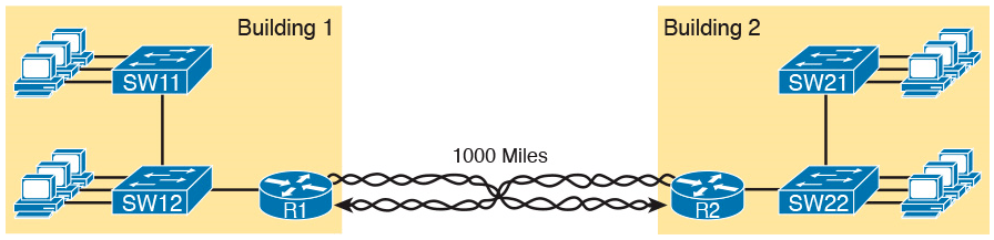
Conceptual View of the Leased-Line Service
Of course, leased lines have many differences compared to an Ethernet crossover cable.
To create such possibly long links, or circuits, a leased line does not actually exist as a single long cable between the two sites.
Instead, the Telco installs a large network of cables and specialized switching devices to create its own computer network. The Telco network creates a service that acts like a crossover cable between two points, but the physical reality is hidden from the customer.
Leased lines come with their own set of terminology as well.
First, the term leased line refers to the fact that the company using the leased line does not own the line, but instead pays a monthly lease fee to use it.
However, many people today use the generic term service provider to refer to a company that provides any form of WAN connectivity, including Internet services.
Given their long history, leased lines have had many names. The table below lists some of those names.
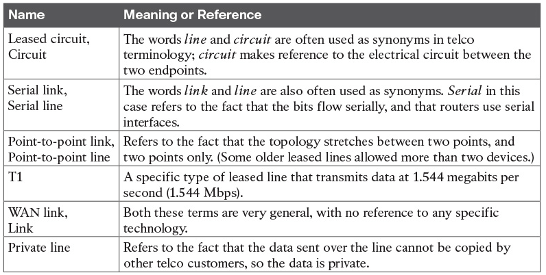
Different Names for a Leased Line
Leased-Line Cabling
To create a leased line, some physical path must exist between the two routers on the ends of the link.
The physical cabling must leave the buildings where each router sits.
However, the telco does not simply install one cable between the two buildings. Instead, it uses what is typically a large and complex network that creates the appearance of a cable between the two routers.
The diagram below gives a little insight into the cabling that could exist inside the telco for a short leased line.
Telcos put their equipment in buildings called central offices (CO). The telco installs cables from the CO to most every other building in the city, expecting to sell services to the people in those buildings one day.
The telco would then configure its switches to use some of the capacity on each cable to send data in both directions, creating the equivalent of a crossover cable between the two routers.
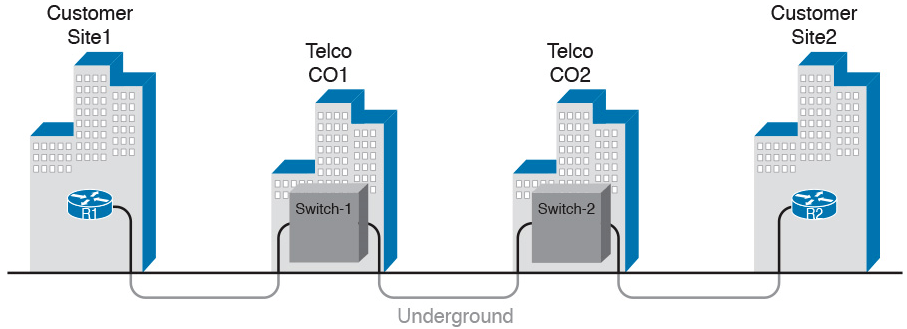
Possible Cabling Inside a Telco for a Short Leased Line
Although what happens inside the telco is completely hidden from the telco customer, enterprise engineers do need to know about the parts of the link that exist inside the customer’s building at the router.
First, each site has customer premises equipment (CPE), which includes the router, serial interface card, and CSU/DSU.
Each router uses a serial interface card that acts somewhat like an Ethernet NIC, sending and receiving data over the physical link.
The physical link requires a function called a channel service unit/data service unit (CSU/DSU). The CSU/DSU can either be integrated into the serial interface card in the router or sit outside the router as an external device.
The diagram below shows the CPE devices, along with the cabling.
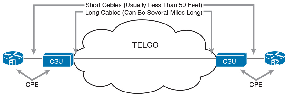
Point-to-Point Leased Line: Components and Terminology
The cabling includes a short serial cable (only if an external CSU/DSU is used) plus the cable installed by the telco for the leased line itself.
The serial cable connects the router serial interface to the external CSU/DSU. (Many cable options exist; the cable just needs to match the connector of the serial interface on one end and the CSU/DSU on the other end.)
The four-wire cable from the telco plugs in to the CSU/DSU, typically using an RJ-48 connector that has the same size and shape as an RJ-45 connector.
Telcos offer a wide variety of speeds for leased lines. However, you cannot pick the exact speed you want; instead, you must pick from a long list of predefined speeds.
Slower-speed links run at multiples of 64 kbps (kilobits per second), while faster links run at multiples of about 1.5 Mbps (megabits per second).
Building a WAN Link in a Lab
One can create the equivalent of a leased line without a real leased line from a telco, and without CSU/DSUs, just using a cabling trick.
First, the serial cables normally used between a router and an external CSU/DSU are called data terminal equipment (DTE) cables.
To create a physical WAN link in a lab, you need two serial cables: one serial DTE cable, plus a similar but slightly different matching data communications equipment (DCE) cable.
The DCE cable has a female connector, while the DTE cable has a male connector, which allows the two cables to be attached directly.
The DCE cable also does the equivalent task of an Ethernet crossover cable by swapping the transmit and receive wire pairs, as shown in the diagram below.
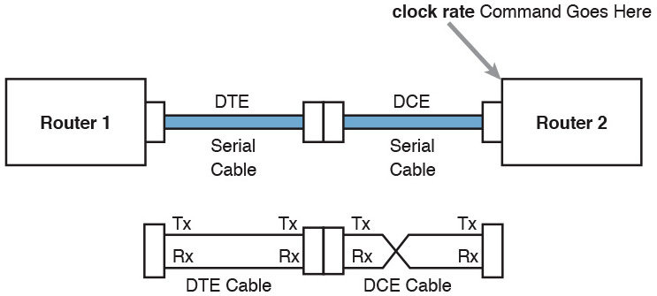
Serial Cabling Uses a DTE Cable and a DCE Cable
The diagram shows the cable details at the top, with the wiring details inside the cable at the bottom.
In particular, at the bottom of the figure, note that the DCE cable swaps the transmit and receive pairs, whereas the DTE serial cable does not, acting as a straight-through cable.
Finally, to make the link work, the router with the DCE cable installed must do one function normally done by the CSU/DSU. The CSU/DSU normally provides a function called clocking, in which it tells the router exactly when to send each bit through signaling over the serial cable.
A router serial interface can provide clocking, and the more recent router software versions automatically supply clocking when the router senses a DCE cable is plugged into the serial port.
Regardless of whether a router has an older or newer software version, you will want to know how to configure serial clocking using the clock rate command
Data-Link Details of Leased Lines
A leased line provides a Layer 1 service.
In other words, it promises to deliver bits between the devices connected to the leased line.
However, the leased line itself does not define a data link layer protocol to be used on the leased line.Because leased lines define only the Layer 1 transmission service, many companies and standards organizations have created data-link protocols to control and use leased lines.
Today, the two most popular data link layer protocols used for leased lines between two routers are High-Level Data Link Control (HDLC) and Point-to-Point Protocol (PPP).
HDLC Basics
All data-link protocols perform a similar role: to control the correct delivery of data over a physical link of a particular type.
For example, the Ethernet data-link protocol uses a destination address field to identify the correct device that should receive the data, and an FCS field that allows the receiving device to determine whether the data arrived correctly. HDLC provides similar functions.
HDLC has less work to do because of the simple point-to-point topology of a point-to-point leased line.
When one router sends an HDLC frame, it can go only one place: to the other end of the link.
So, while HDLC has an address field, the destination is implied.
HDLC has other fields and functions similar to Ethernet as well.
The table below lists the HDLC fields, with the similar Ethernet header/trailer field.
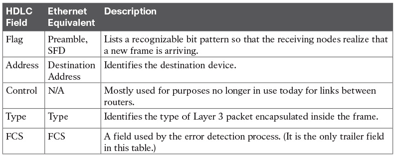
Comparing HDLC Header Fields to Ethernet
HDLC exists today as a standard of the International Organization for Standardization (ISO), the same organization that brought us the OSI model.
However, ISO standard HDLC does not have a Type field, and routers need to know the type of packet inside the frame. So, Cisco routers use a Cisco-proprietary variation of HDLC that adds a Type field, as shown in the diagram below.
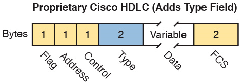
HDLC Framing
How Routers Use a WAN Data Link
Today, most leased lines connect to routers, and routers focus on delivering packets to a destination host.
However, routers physically connect to both LANs and WANs, with those LANs and WANs requiring that data be sent inside data-link frames.
So, now that you know a little about HDLC, it helps to think about how routers use the HDLC protocol when sending data.
First, the TCP/IP network layer focuses on forwarding IP packets from the sending host to the destination host. The underlying LANs and WANs just act as a way to move the packets to the next router or end-user device. The diagram below shows that network layer perspective.
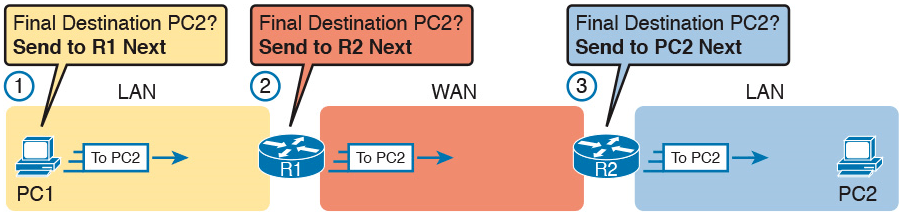
IP Routing Logic over LANs and WANs
Following the steps in the figure, for a packet sent by PC1 to PC2’s IP address:
- PC1’s network layer (IP) logic tells it to send the packet to a nearby router (R1).
- Router R1’s network layer logic tells it to forward (route) the packet out the leased line to Router R2 next.
- Router R2’s network layer logic tells it to forward (route) the packet out the LAN link to PC2 next.
While the diagram above shows the network layer logic, the PCs and routers must rely on the LANs and WANs in the diagram to actually move the bits in the packet.
The diagram below shows the same figure, with the same packet, but this time showing some of the data link layer logic used by the hosts and routers.
Basically, three separate data link layer steps encapsulate the packet, inside a data-link frame, over three hops through the internetwork: from PC1 to R1, from R1 to R2, and from R2 to PC2
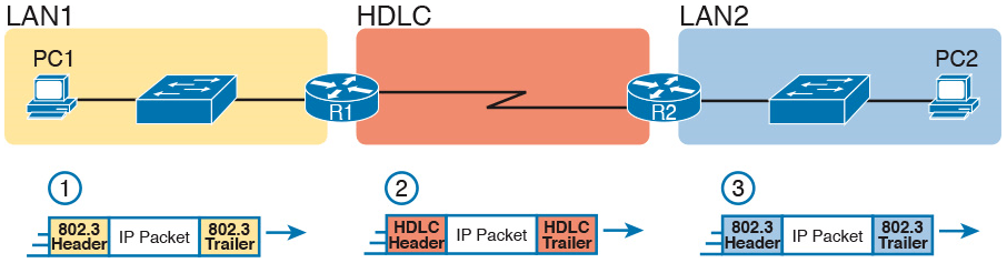
General Concept of Routers De-encapsulating and Re-encapsulating IP Packets
Following the steps in the diagram, again for a packet sent by PC1 to PC2’s IP address:
- To send the IP packet to Router R1 next, PC1 encapsulates the IP packet in an Ethernet frame that has the destination MAC address of R1.
- Router R1 de-encapsulates (removes) the IP packet from the Ethernet frame, encapsulates the packet into an HDLC frame using an HDLC header and trailer, and forwards the HDLC frame to Router R2 next.
- Router R2 de-encapsulates (removes) the IP packet from the HDLC frame, encapsulates the packet into an Ethernet frame that has the destination MAC address of PC2, and forwards the Ethernet frame to PC2.
In summary, a leased line with HDLC creates a WAN link between two routers so that they can forward packets for the devices on the attached LANs.
The leased line itself provides the physical means to transmit the bits, in both directions. The HDLC frames provide the means to encapsulate the network layer packet correctly so that it crosses the link between routers.
Leased lines have many benefits that have led to their relatively long life in the WAN marketplace. These lines are simple for the customer, are widely available, are of high quality, and are private.
However, they do have some negatives as well compared to newer WAN technologies, including a higher cost and typically longer lead times to get the service installed.
Ethernet as a WAN Technology
For the first several decades of the existence of Ethernet, Ethernet was only appropriate for LANs.
The restrictions on cable lengths and devices might allow a LAN that stretched a kilometer or two, to support a campus LAN, but that was the limit.
As time passed, the IEEE improved Ethernet standards in ways that made Ethernet a reasonable WAN technology.
For example, the 1000BASE-LX standard uses single-mode fiber cabling, with support for a 5-km cable length; the 1000BASE-ZX standard supports an even longer 70-km cable length.
As time went by, and as the IEEE improved cabling distances for fiber Ethernet links, Ethernet became a reasonable WAN technology.
Today, in this second decade of the twenty-first century, many WAN service providers (SP) offer WAN services that take advantage of Ethernet.
SPs offer a wide variety of these Ethernet WAN services, with many different names. But all of them use a similar model, with Ethernet used between the customer site and the SP’s network, as shown in the diagram below.
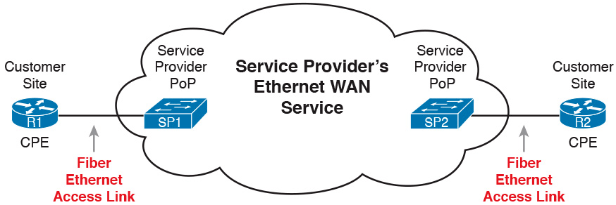
Fiber Ethernet Link to Connect a CPE Router to a Service Provider’s WAN
The customer connects to an Ethernet link using a router interface. The (fiber) Ethernet link leaves the customer building and connects to some nearby SP location called a point of presence (PoP).
Instead of a telco switch, the SP uses an Ethernet switch. Inside the SP’s network, the SP uses any technology that it wants to create the specific Ethernet WAN services.
Ethernet WANs that Create a Layer 2 Service
The WAN services implied by the previous diagram include a broad number of services, with a lot of complex networking concepts needed to understand those services.
The one Ethernet WAN service goes by two names: Ethernet emulation and Ethernet over MPLS (EoMPLS).
Ethernet emulation is a general term, meaning that the service acts like one Ethernet link.
EoMPLS refers to Multiprotocol Label Switching (MPLS), which is one technology that can be used inside the SP’s cloud.
The EoMPLS service provides:
- A point-to-point connection between two customer devices
- Behavior as if a fiber Ethernet link existed between the two devices
So, if you can imagine two routers, with a single Ethernet link between the two routers, you understand what this particular EoMPLS service does.
The diagram below shows the idea. In this case, the two routers, R1 and R2, connect with an EoMPLS service instead of a serial link. The routers use Ethernet interfaces, and they can send data in both directions at the same time. Physically, each router actually connects to some SP PoP, but logically, the two routers can send Ethernet frames to each other over the link.

EoMPLS Acting Like a Simple Ethernet Link Between Two Routers
How Routers Route IP Packets Using Ethernet Emulation
WANs, by their very nature, give IP routers a way to forward IP packets from a LAN at one site, over the WAN, and to another LAN at another site.
Routing over an EoMPLS WAN link still uses the WAN like a WAN, as a way to forward IP packets from one site to another.
However, the WAN link happens to use the same Ethernet protocols as the Ethernet LAN links at each site.
The EoMPLS link uses Ethernet for both Layer 1 and Layer 2 functions. That means the link uses the same familiar Ethernet header and trailer, as shown in the middle the diagram below.
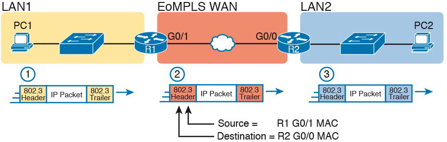
Routing over an EoMPLS Link
All three routing steps use the same Ethernet (802.3) protocol. However, note that each frame’s data-link header and trailer are different.
Each router discards the old data-link header/trailer and adds a new set, as described in these steps.
- To send the IP packet to Router R1 next, PC1 encapsulates the IP packet in an Ethernet frame that has the destination MAC address of R1.
- Router R1 de-encapsulates (removes) the IP packet from the Ethernet frame and encapsulates the packet into a new Ethernet frame, with a new Ethernet header and trailer. The destination MAC address is R2’s G0/0 MAC address, and the source MAC address is R1’s G0/1 MAC address. R1 forwards this frame over the EoMPLS service to R2 next.
- Router R2 de-encapsulates (removes) the IP packet from the Ethernet frame, encapsulates the packet into an Ethernet frame that has the destination MAC address of PC2, and forwards the Ethernet frame to PC2.
Accessing the Internet
Two other popular WAN technologies used to gain access to the Internet: digital subscriber line (DSL) and cable.
These two WAN technologies do not replace leased lines in all cases, but they do play an important role in the specific case of creating a WAN connection between a home or office and the Internet.
The Internet as a Large WAN
The Internet is an amazing cultural phenomenon. Most of us use it every day. We post messages on social media sites, we search for information using a search engine like Google, and we send emails.
We use apps on our phones to pull down information, like weather reports, maps, and movie reviews.
We use the Internet to purchase physical products and to buy and download digital products like music and videos. The Internet has created completely new things to do and changed the old ways of living life compared to a generation ago.
However, if you instead focus on the networking technology that creates the Internet, the Internet is simply one huge TCP/IP network.
In fact, the name “Internet” comes from the core network layer protocol: Internet Protocol. The Internet includes many LANs, and because the Internet spans the globe, it of course needs WAN links to connect different sites.
As a network of networks, the Internet is actually owned by countless companies and people.
The Internet includes most every enterprise TCP/IP network and a huge number of home-based networks, as well as a huge number of individuals from their phones and other wireless devices, as shown in the diagram below.
Internet with Enterprise, Home, and Phone Subscribers
The middle of the Internet, called the Internet core, exists as LANs and WANs owned and operated by Internet service providers (ISP).
(The diagram above shows the Internet core as a cloud, because network diagrams show a cloud when hiding the details of a part of the network.)
ISPs cooperate to create a mesh of links between each other in the Internet core, so that no matter through which ISP a particular company or person connects, some path exists to every device.
The diagram below shows a slightly different version, in this case showing the concept of the Internet core: ISP networks that connect to both their customers as well as each other, so that IP packets can flow from every customer of every ISP to every other customer of every other ISP.
Internet Core with Multiple ISPs and Telcos
Internet Access (WAN) Links
The Internet also happens to use a huge number of WAN links.
All of those lines connecting an enterprise or home to one of the ISPs in above diagram represent some kind of WAN link that uses a cable, while the phones create their WAN link using wireless technology.
These links usually go by the name Internet access link.
Historically, businesses tend to use one set of WAN technologies as Internet access links, while home-based consumers use others.
Businesses often use leased lines, connecting a router at the business to a router at the ISP. The top of the diagram below shows just such an example.
Three Examples of Internet Access Links
Consumers often use technologies like DSL and cable for Internet access links.
These technologies use cabling that is already installed in most homes, making these services somewhat inexpensive for home users.
DSL uses the analog phone lines that are already installed in homes, while cable Internet uses the cable TV (CATV) cable.
While DSL and cable are popular with consumers, many businesses use these technologies for Internet access.
All three of the Internet access technologies in the diagram above happen to use a pair of routers: one at the customer side of the WAN link and one at the ISP side.
The routers will continue to think about network layer logic, of sending IP packets to their destination by forwarding the packets to the next router.
However, the physical and data link layer details on the WAN link differ as compared to leased lines.
Digital Subscriber Line
Digital subscriber line (DSL) creates a relatively short (miles long, not tens of miles) high-speed link WAN between a telco customer and an ISP.
To do so, it uses the same single-pair telephone line used for a typical home phone line.
DSL, as a technology, does not try to replace leased lines, which run between any two sites, for potentially very long distances.
DSL instead just provides a short physical link from a home to the telco’s network, allowing access to the Internet.
First, to get an idea about the cabling, think of a typical home. Each home has one phone line that runs from a nearby telco CO to the home.
As shown on the left side of diagram below, the telephone wiring splits out and terminates at several wall plates, often with RJ-11 ports that are a slightly skinnier cousin of the RJ-45 connector.

Typical Voice Cabling Concepts in the United States
Next, think about the telephone line and the equipment at the CO.
Sometime in the past, the telco installed all the telephone lines from its local CO to each neighborhood, apartment, and so on.
At the CO, each line connects to a port on a telco switch. This switch supports the ability to set up voice calls, take them down, and forward the voice through the worldwide voice network, called the public switched telephone network, or PSTN.
To add DSL service at the home int the above diagram, two changes need to be made.
First, you need to add DSL-capable devices at the home.
Second, the telco has to add DSL equipment at the CO.
Together, the DSL equipment at each side of the local telephone line can send data while still supporting the same voice traffic.
The left side of below diagram shows the changes.

Wiring and Devices for a Home DSL Link
A new DSL modem now connects to a spare phone outlet.
The DSL modem follows the DSL physical and data link layer standards to send data to/from the telco.
The home now has a small LAN, implemented with a consumer-grade router, which often includes an Ethernet switch and possibly a wireless LAN access point.
(Note that the telephones may now also need a short extra cable with a filter in it, installed at the wall jack, to filter out the sounds of the higher electrical frequencies used for DSL.)
The home-based router on the left must be able to send data to/from the Internet.
To make that happen, the telco CO uses a product called a DSL access multiplexer (DSLAM).
The DSLAM splits out the data over to the router on the lower right, which completes the connection to the Internet. The DSLAM also splits out the voice signals over to the voice switch on the upper right.
DSL gives telcos a useful high-speed Internet service to offer their customers.
Telcos have had other offerings that happen to use the same telephone line for data, but these options ran much slower than DSL.
DSL supports asymmetric speeds, meaning that the transmission speed from the ISP toward the home (downstream) is much faster than the transmissions toward the ISP (upstream).
Asymmetric speeds work better for consumer Internet access from the home, because clicking a web page sends only a few hundred bytes upstream into the Internet, but can trigger many megabytes of data to be delivered downstream to the home.
Cable Internet
Cable Internet creates an Internet access service which, when viewed generally rather than specifically, has many similarities to DSL.
Like DSL, cable Internet takes full advantage of existing cabling, using the existing cable TV (CATV) cable to send data.
Like DSL, cable Internet uses asymmetric speeds, sending data faster downstream than upstream, which works better than symmetric speeds for most consumer locations.
And like DSL, cable Internet does not attempt to replace long leased lines between any two sites, instead focusing on the short WAN links from a customer to an ISP.
Cable Internet also uses the same basic in-home cabling concepts as does DSL.
The diagram below shows a diagram similar to DSL, but with the DSL details replaced with cable Internet details.
The telephone line has been replaced with coaxial cable from the CATV company, and the DSL modem has been replaced by a cable modem.
Otherwise, the details in the home follow the same overall plan.
Wiring and Devices for a Home Cable Internet Link
On the CATV company side of the cable Internet service, the CATV company has to split out the data and video, as shown on the right side of the diagram.
Data flows to the lower right, through a router, while video comes in from video dishes for distribution out to the TVs in people’s homes.
Cable Internet service and DSL directly compete for consumer and small-business Internet access.
Generally speaking, while both offer high speeds, cable Internet typically runs at faster speeds than DSL, with DSL providers keeping their prices a little lower to compete.
Both support asymmetric speeds, and both provide an “always on” service, in that you can communicate with the Internet without the need to first take some action to start the Internet connection.

Fundamentals of Ethernet LANs
INTERNOLD NETWORKS CCNA LIVE WEBCLASS (INCLW)
Fundamentals of Ethernet LANs
Contents
Fundamentals of Ethernet LANs
Most enterprise computer networks can be separated into two general types of technology: local-area networks (LAN) and wide-area networks (WAN).
LANs typically connect nearby devices: devices in the same room, in the same building, or in a campus of buildings.
In contrast, WANs connect devices that are typically relatively far apart.
Together, LANs and WANs create a complete enterprise computer network, working together to do the job of a computer network: delivering data from one device to another
Many types of LANs have existed over the years, but today’s networks use two general types of LANs: Ethernet LANs and wireless LANs.
Ethernet LANs happen to use cables for the links between nodes, and because many types of cables use copper wires, Ethernet LANs are often called wired LANs.
In comparison, wireless LANs do not use wires or cables, instead using radio waves for the links between nodes.
Overview of LANs
The term Ethernet refers to a family of LAN standards that together define the physical and data link layers of the world’s most popular wired LAN technology.
The standards, defined by the Institute of Electrical and Electronics Engineers (IEEE), define the cabling, the connectors on the ends of the cables, the protocol rules, and everything else required to create an Ethernet LAN.
SOHO LANs
To begin, first think about a small office/home office (SOHO) LAN today, specifically a LAN that uses only Ethernet LAN technology.
First, the LAN needs a device called an Ethernet LAN switch, which provides many physical ports into which cables can be connected.
An Ethernet uses Ethernet cables, which is a general reference to any cable that conforms to any of several Ethernet standards.
The LAN uses Ethernet cables to connect different Ethernet devices or nodes to one of the switch’s Ethernet ports.
Below diagram shows a drawing of a SOHO Ethernet LAN. The figure shows a single LAN switch, five cables, and five other Ethernet nodes: three PCs, a printer, and one network device called a router. (The router connects the LAN to the WAN, in this case to the Internet.)

Small Ethernet-only SOHO LAN
Although above diagram shows a simple Ethernet LAN, many SOHO Ethernet LANs today combine the router and switch into a single device.
Vendors sell consumer-grade integrated networking devices that work as a router and Ethernet switch, as well as doing other functions.
These devices typically have “router” on the packaging, but many models also have four-port or eight-port Ethernet LAN switch ports built in to the device
Typical SOHO LANs today also support wireless LAN connections.
Ethernet defines wired LAN technology only; in other words, Ethernet LANs use cables.
However, you can build one LAN that uses both Ethernet LAN technology as well as wireless LAN technology, which is also defined by the IEEE.
Wireless LANs, defined by the IEEE using standards that begin with 802.11, use radio waves to send the bits from one node to the next.
Most wireless LANs rely on yet another networking device: a wireless LAN access point (AP).
The AP acts somewhat like an Ethernet switch, in that all the wireless LAN nodes communicate with the Ethernet switch by sending and receiving data with the wireless AP.
Of course, as a wireless device, the AP does not need Ethernet ports for cables, other than for a single Ethernet link to connect the AP to the Ethernet LAN, as shown below.

Small Wired and Wireless SOHO LAN
Note that this diagram shows the router, Ethernet switch, and wireless LAN access point as three separate devices so that you can better understand the different roles.
However, most SOHO networks today would use a single device, often labeled as a “wireless router,” that does all these functions.
Enterprise LANs
Enterprise networks have similar needs compared to a SOHO network, but on a much larger scale.
For example, enterprise Ethernet LANs begin with LAN switches installed in a wiring closet behind a locked door on each floor of a building.
The electricians install the Ethernet cabling from that wiring closet to cubicles and conference rooms where devices might need to connect to the LAN.
At the same time, most enterprises also support wireless LANs in the same space, to allow people to roam around and still work and to support a growing number of devices that do not have an Ethernet LAN interface.
Below is a conceptual view of a typical enterprise LAN in a three-story building.
Each floor has an Ethernet LAN switch and a wireless LAN AP.
To allow communication between floors, each per-floor switch connects to one centralized distribution switch.
For example, PC3 can send data to PC2, but it would first flow through switch SW3 to the first floor to the distribution switch (SWD) and then back up through switch SW2 on the second floor.

Single-Building Enterprise Wired and Wireless LAN
The figure also shows the typical way to connect a LAN to a WAN using a router. LAN switches and wireless access points work to create the LAN itself. Routers connect to both the LAN and the WAN.
To connect to the LAN, the router simply uses an Ethernet LAN interface and an Ethernet cable, as shown on the lower right of the diagram above.
Variety of Ethernet Physical Layer Standards
The term Ethernet refers to an entire family of standards.
Some standards define the specifics of how to send data over a particular type of cabling, and at a particular speed.
Other standards define protocols, or rules, that the Ethernet nodes must follow to be a part of an Ethernet LAN.
All these Ethernet standards come from the IEEE and include the number 802.3 as the beginning part of the standard name.
Ethernet supports a large variety of options for physical Ethernet links given its long history over the last 40 or so years.
Today, Ethernet includes many standards for different kinds of optical and copper cabling, and for speeds from 10 megabits per second (Mbps) up to 100 gigabits per second (Gbps).
The standards also differ as far as the types of cabling and the allowed length of the cabling.
The most fundamental cabling choice has to do with the materials used inside the cable for the physical transmission of bits: either copper wires or glass fibers.
The use of unshielded twisted-pair (UTP) cabling saves money compared to optical fibers, with Ethernet nodes using the wires inside the cable to send data over electrical circuits.
Fiber-optic cabling, the more expensive alternative, allows Ethernet nodes to send light over glass fibers in the center of the cable.
Although more expensive, optical cables typically allow longer cabling distances between nodes.
To be ready to choose the products to purchase for a new Ethernet LAN, a network engineer must know the names and features of the different Ethernet standards supported in Ethernet products. The IEEE defines Ethernet physical layer standards using a couple of naming conventions.
The formal name begins with 802.3 followed by some suffix letters.
The IEEE also uses more meaningful shortcut names that identify the speed, as well as a clue about whether the cabling is UTP (with a suffix that includes T) or fiber (with a suffix that includes X).
The table below lists a few Ethernet physical layer standards.

Types of Ethernet
First, the table lists enough names so that you get a sense of the IEEE naming conventions.
It also lists the four most common standards that use UTP cabling, because this book’s discussion of Ethernet focuses mainly on the UTP options.
Consistent Behavior over All Links Using the Ethernet Data Link Layer
While the physical layer standards focus on sending bits over a cable, the Ethernet data-link protocols focus on sending an Ethernet frame from source to destination Ethernet node. From a data-link perspective, nodes build and forward frames. The term frame specifically refers to the header and trailer of a data-link protocol, plus the data encapsulated inside that header and trailer.
The diagram below shows an example of the process. In this case, PC1 sends an Ethernet frame to PC3. The frame travels over a UTP link to Ethernet switch SW1, then over fiber links to Ethernet switches SW2 and SW3, and finally over another UTP link to PC3. Note that the bits actually travel at four different speeds in this example: 10 Mbps, 1 Gbps, 10 Gbps, and 100 Mbps, respectively.

So, what is an Ethernet LAN? It is a combination of user devices, LAN switches, and different kinds of cabling. Each link can use different types of cables, at different speeds. However, they all work together to deliver Ethernet frames from the one device on the LAN to some other device.
Building Physical Ethernet Networks with UTP
Before the Ethernet network as a whole can send Ethernet frames between user devices, each node must be ready and able to send data over an individual physical link.
The three most commonly used Ethernet standards: 10BASE-T (Ethernet), 100BASE-T (Fast Ethernet, or FE), and 1000BASE-T (Gigabit Ethernet, or GE) which respectively uses the cables for 10-Mbps, 100-Mbps, and 1000-Mbps Ethernet.
Transmitting Data Using Twisted Pairs
While it is true that Ethernet sends data over UTP cables, the physical means to send the data uses electricity that flows over the wires inside the UTP cable.
To better understand how Ethernet sends data using electricity, break the idea down into two parts: how to create an electrical circuit and then how to make that electrical signal communicate 1s and 0s.
First, to create one electrical circuit, Ethernet defines how to use the two wires inside a single twisted pair of wires, as shown on the diagram below.

Creating One Electrical Circuit over One Pair to Send in One Direction
The diagram does not show a UTP cable between two nodes, but instead shows two individual wires that are inside the UTP cable.
An electrical circuit requires a complete loop, so the two nodes, using circuitry on their Ethernet ports, connect the wires in one pair to complete a loop, allowing electricity to flow.
Note that in an actual UTP cable, the wires will be twisted together, instead of being parallel.
The twisting helps solve some important physical transmission issues.
When electrical current passes over any wire, it creates electromagnetic interference (EMI) that interferes with the electrical signals in nearby wires, including the wires in the same cable. (EMI between wire pairs in the same cable is called crosstalk.)
Twisting the wire pairs together helps cancel out most of the EMI, so most networking physical links that use copper wires use twisted pairs.
Breaking Down a UTP Ethernet Link
The term Ethernet link refers to any physical cable between two Ethernet nodes.
To learn about how a UTP Ethernet link works, it helps to break down the physical link into those basic pieces, as shown below: the cable itself, the connectors on the ends of the cable, and the matching ports on the devices into which the connectors will be inserted.

Basic Components of an Ethernet Link
First, think about the UTP cable itself. The cable holds some copper wires, grouped as twisted pairs.
The 10BASE-T and 100BASE-T standards require two pairs of wires, while the 1000BASE-T standard requires four pairs.
Each wire has a color-coded plastic coating, with the wires in a pair having a color scheme.
For example, for the blue wire pair, one wire’s coating is all blue, while the other wire’s coating is blue-and-white striped.
Many Ethernet UTP cables use an RJ-45 connector on both ends.
The RJ-45 connector has eight physical locations into which the eight wires in the cable can be inserted, called pin positions, or simply pins.
These pins create a place where the ends of the copper wires can touch the electronics inside the nodes at the end of the physical link so that electricity can flow.
To complete the physical link, the nodes each need an RJ-45 Ethernet port that matches the RJ-45 connectors on the cable so that the connectors on the ends of the cable can connect to each node.
Computers often include this RJ-45 Ethernet port as part of a network interface card (NIC), which can be an expansion card on the PC or can be built in to the system itself. Switches typically have many RJ-45 ports because switches give user devices a place to connect to the Ethernet LAN.

RJ-45 Connectors and Ports
The diagram above shows a connector on the left and ports on the right. The left shows the eight pin positions in the end of the RJ-45 connector. The upper right shows an Ethernet NIC that is not yet installed in a computer.
The lower-right part of the figure shows the side of a Cisco 2960 switch, with multiple RJ-45 ports, allowing multiple devices to easily connect to the Ethernet network.
Finally, while RJ-45 connectors with UTP cabling can be common, Cisco LAN switches often support other types of connectors as well. When you buy one of the many models of Cisco switches, you need to think about the mix and numbers of each type of physical ports you want on the switch.
To give its customers flexibility as to the type of Ethernet links, even after the customer has bought the switch, Cisco switches include some physical ports whose port hardware (the transceiver) can be changed later, after you purchase the switch.
For example, below shows a photo of a Cisco switch with one of the swappable transceivers. In this case, the figure shows an enhanced small form-factor pluggable (SFP+) transceiver, which runs at 10 Gbps, just outside two SFP+ slots on a Cisco 3560CX switch. The SFP+ itself is the silver colored part below the switch, with a black cable connected to it.

10Gbps SFP+ with Cable Sitting Just Outside a Catalyst 3560CX Switch
UTP Cabling Pinouts for 10BASE-T and 100BASE-T
Straight-Through Cable Pinout
10BASE-T and 100BASE-T use two pairs of wires in a UTP cable, one for each direction, as shown in diagram below.
The figure shows four wires, all of which sit inside a single UTP cable that connects a PC and a LAN switch. In this example, the PC on the left transmits using the top pair, and the switch on the right transmits using the bottom pair.

For correct transmission over the link, the wires in the UTP cable must be connected to the correct pin positions in the RJ-45 connectors.
For example, in the diagram above, the transmitter on the PC on the left must know the pin positions of the two wires it should use to transmit. Those two wires must be connected to the correct pins in the RJ-45 connector on the switch, so that the switch’s receiver logic can use the correct wires.
To understand the wiring of the cable—which wires need to be in which pin positions on both ends of the cable—you need to first understand how the NICs and switches work.
As a rule, Ethernet NIC transmitters use the pair connected to pins 1 and 2; the NIC receivers use a pair of wires at pin positions 3 and 6. LAN switches, knowing those facts about what Ethernet NICs do, do the opposite: Their receivers use the wire pair at pins 1 and 2, and their transmitters use the wire pair at pins 3 and 6.
To allow a PC NIC to communicate with a switch, the UTP cable must also use a straight-through cable pinout.
The term pinout refers to the wiring of which color wire is placed in each of the eight numbered pin positions in the RJ-45 connector.
An Ethernet straight-through cable connects the wire at pin 1 on one end of the cable to pin 1 at the other end of the cable; the wire at pin 2 needs to connect to pin 2 on the other end of the cable; pin 3 on one end connects to pin 3 on the other, and so on.
Also, it uses the wires in one wire pair at pins 1 and 2, and another pair at pins 3 and 6.

Ethernet LAN Forwards a Data-Link Frame over Many Types of Link
The diagram below shows one final perspective on the straight-through cable pinout.
In this case, PC Larry connects to a LAN switch.
Note that the diagram again does not show the UTP cable, but instead shows the wires that sit inside the cable, to emphasize the idea of wire pairs and pins.

Ethernet Straight-Through Cable Concept
Crossover Cable Pinout
A straight-through cable works correctly when the nodes use opposite pairs for transmitting data.
However, when two like devices connect to an Ethernet link, they both transmit on the same pins.
In that case, you then need another type of cabling pinout called a crossover cable.
The crossover cable pinout crosses the pair at the transmit pins on each device to the receive pins on the opposite device.
This concept is much clearer with a diagram below.

Crossover Ethernet Cable
The figure shows what happens on a link between two switches. The two switches both transmit on the pair at pins 3 and 6, and they both receive on the pair at pins 1 and 2. So, the cable must connect a pair at pins 3 and 6 on each side to pins 1 and 2 on the other side, connecting to the other node’s receiver logic. The top of the figure shows the literal pinouts, and the bottom half shows a conceptual diagram.
Choosing the Right Cable Pinouts
- Crossover cable: If the endpoints transmit on the same pin pair
- Straight-through cable: If the endpoints transmit on different pin pairs

10BASE-T and 100BASE-T Pin Pairs Used
The diagram below shows a LAN in a single building. In this case, several straight-through cables are used to connect PCs to switches. In addition, the cables connecting the switches require crossover cables.

Typical Uses for Straight-Through and Crossover Ethernet Cables
NOTE: If you have some experience with installing LANs, you might be thinking that you have used the wrong cable before (straight-through or crossover) but the cable worked. Cisco switches have a feature called auto-mdix that notices when the wrong cable is used and automatically changes its logic to make the link work.
However, for the exams, be ready to identify whether the correct cable is shown in the diagrams.
UTP Cabling Pinouts for 1000BASE-T
1000BASE-T (Gigabit Ethernet) differs from 10BASE-T and 100BASE-T as far as the cabling and pinouts.
First, 1000BASE-T requires four wire pairs.
Second, it uses more advanced electronics that allow both ends to transmit and receive simultaneously on each wire pair.
However, the wiring pinouts for 1000BASE-T work almost identically to the earlier standards, adding details for the additional two pairs.
The straight-through cable connects each pin with the same numbered pin on the other side, but it does so for all eight pins—pin 1 to pin 1, pin 2 to pin 2, up through pin 8.
It keeps one pair at pins 1 and 2 and another at pins 3 and 6, just like in the earlier wiring. It adds a pair at pins 4 and 5 and the final pair at pins 7 and 8 as shown in the diagram below.
Ethernet LAN Forwards a Data-Link Frame over Many Types of Link
The Gigabit Ethernet crossover cable crosses the same two-wire pairs as the crossover cable for the other types of Ethernet (the pairs at pins 1,2 and 3,6). It also crosses the two new pairs as well (the pair at pins 4,5 with the pair at pins 7,8).
Sending Data in Ethernet Networks
Although physical layer standards vary quite a bit, other parts of the Ethernet standards work the same way, regardless of the type of physical Ethernet link.
Ethernet Data-Link Protocols
One of the most significant strengths of the Ethernet family of protocols is that these protocols use the same data-link standard.
The Ethernet data-link protocol defines the Ethernet frame: an Ethernet header at the front, the encapsulated data in the middle, and an Ethernet trailer at the end as shown in the diagrams below with the description of each field.

Commonly Used Ethernet Frame Format

IEEE 802.3 Ethernet Header and Trailer Fields
Ethernet Addressing
The source and destination Ethernet address fields play a huge role in how Ethernet LANs work.
The general idea for each is relatively simple: The sending node puts its own address in the source address field and the intended Ethernet destination device’s address in the destination address field.
The sender transmits the frame, expecting that the Ethernet LAN, as a whole, will deliver the frame to that correct destination.
Ethernet addresses, also called Media Access Control (MAC) addresses, are 6-byte-long (48-bit-long) binary numbers.
MAC addresses as 12-digit hexadecimal numbers.
Cisco devices typically add some periods to the number for easier readability as well; for example, a Cisco switch might list a MAC address as 0000.0C12.3456.
Most MAC addresses represent a single NIC or other Ethernet port, so these addresses are often called a unicast Ethernet address.
The term unicast is simply a formal way to refer to the fact that the address represents one interface to the Ethernet LAN. (This term also contrasts with two other types of Ethernet addresses, broadcast and multicast, which will be defined later.)
The entire idea of sending data to a destination unicast MAC address works well, but it works only if all the unicast MAC addresses are unique.
If two NICs tried to use the same MAC address, there could be confusion.
If two PCs on the same Ethernet tried to use the same MAC address, to which PC should frames sent to that MAC address be delivered?
Ethernet solves this problem using an administrative process so that, at the time of manufacture, all Ethernet devices are assigned a universally unique MAC address.
Before a manufacturer can build Ethernet products, it must ask the IEEE to assign the manufacturer a universally unique 3-byte code, called the organizationally unique identifier (OUI).
The manufacturer agrees to give all NICs (and other Ethernet products) a MAC address that begins with its assigned 3-byte OUI.
The manufacturer also assigns a unique value for the last 3 bytes, a number that manufacturer has never used with that OUI. As a result, the MAC address of every device in the universe is unique.
The diagram below shows the structure of the unicast MAC address, with the OUI.

Structure of Unicast Ethernet Addresses
Ethernet addresses go by many names:
- LAN address
- Ethernet address
- hardware address
- burned-in address (BIA)
- physical address
- universal address
- MAC address.
The term burned-in address (BIA) refers to the idea that a permanent MAC address has been encoded (burned into) the ROM chip on the NIC.
As another example, the IEEE uses the term universal address to emphasize the fact that the address assigned to a NIC by a manufacturer should be unique among all MAC addresses in the universe.
Broadcast and Multicast Address
In addition to unicast addresses, Ethernet also uses group addresses.
Group addresses identify more than one LAN interface card. A frame sent to a group address might be delivered to a small set of devices on the LAN, or even to all devices on the LAN.
In fact, the IEEE defines two general categories of group addresses for Ethernet:
- Broadcast address: Frames sent to this address should be delivered to all devices on the Ethernet LAN. It has a value of FFFF.FFFF.FFFF.
- Multicast addresses: Frames sent to a multicast Ethernet address will be copied and forwarded to a subset of the devices on the LAN that volunteers to receive frames sent to a specific multicast address.
The diagram below summarizes most of the details about MAC addresses.

LAN MAC Address Terminology and Features
Identifying Network Layer Protocols with the Ethernet Type Field
While the Ethernet header’s address fields play an important and more obvious role in Ethernet LANs, the Ethernet Type field plays a much less obvious role.
The Ethernet Type field, or EtherType, sits in the Ethernet data link layer header, but its purpose is to directly help the network processing on routers and hosts.
Basically, the Type field identifies the type of network layer (Layer 3) packet that sits inside the Ethernet frame.
First, think about what sits inside the data part of the Ethernet frame shown in the diagram below.
Typically, it holds the network layer packet created by the network layer protocol on some device in the network.
Over the years, those protocols have included IBM Systems Network Architecture (SNA), Novell NetWare, Digital Equipment Corporation’s DECnet, and Apple Computer’s AppleTalk.
Today, the most common network layer protocols are both from TCP/IP: IP version 4 (IPv4) and IP version 6 (IPv6).
The original host has a place to insert a value (a hexadecimal number) to identify the type of packet encapsulated inside the Ethernet frame.
However, what number should the sender put in the header to identify an IPv4 packet as the type? Or an IPv6 packet?
As it turns out, the IEEE manages a list of EtherType values, so that every network layer protocol that needs a unique EtherType value can have a number.
The sender just has to know the list. (To view the complete list; just go to www.ieee.org and search for EtherType or click here.)
For example, a host can send one Ethernet frame with an IPv4 packet and the next Ethernet frame with an IPv6 packet.
Each frame would have a different Ethernet Type field value, using the values reserved by the IEEE, as shown in the diagram below.

Use of Ethernet Type Field
Error Detection with FCS
Ethernet also defines a way for nodes to find out whether a frame’s bits changed while crossing over an Ethernet link. (Usually, the bits could change because of some kind of electrical interference, or a bad NIC.)
Ethernet, like most data-link protocols, uses a field in the data-link trailer for the purpose of error detection.
The Ethernet Frame Check Sequence (FCS) field in the Ethernet trailer—the only field in the Ethernet trailer—gives the receiving node a way to compare results with the sender, to discover whether errors occurred in the frame.
The sender applies a complex math formula to the frame before sending it, storing the result of the formula in the FCS field.
The receiver applies the same math formula to the received frame. The receiver then compares its own results with the sender’s results. If the results are the same, the frame did not change; otherwise, an error occurred and the receiver discards the frame.
Note that error detection does not also mean error recovery.
Ethernet defines that the errored frame should be discarded, but Ethernet does not attempt to recover the lost frame.
Other protocols, notably TCP, recover the lost data by noticing that it is lost and sending the data again.
Sending Ethernet Frames with Switches and Hubs
Ethernet LANs behave slightly differently depending on whether the LAN has mostly modern devices, in particular, LAN switches instead of some older LAN devices called LAN hubs.
Basically, the use of more modern switches allows the use of full-duplex logic, which is much faster and simpler than half-duplex logic, which is required when using hubs.
Sending in Modern Ethernet LANs Using Full Duplex
Modern Ethernet LANs use a variety of Ethernet physical standards, but with standard Ethernet frames that can flow over any of these types of physical links.
Each individual link can run at a different speed, but each link allows the attached nodes to send the bits in the frame to the next node. They must work together to deliver the data from the sending Ethernet node to the destination node.
The process is relatively simple, on purpose; the simplicity lets each device send a large number of frames per second. The diagram below shows an example in which PC1 sends an Ethernet frame to PC2.

Example of Sending Data in a Modern Ethernet LAN
The steps in the diagram corresponds to below.
- PC1 builds and sends the original Ethernet frame, using its own MAC address as the source address and PC2’s MAC address as the destination address.
- Switch SW1 receives and forwards the Ethernet frame out its G0/1 interface (short for Gigabit interface 0/1) to SW2.
- Switch SW2 receives and forwards the Ethernet frame out its F0/2 interface (short for Fast Ethernet interface 0/2) to PC2.
- PC2 receives the frame, recognizes the destination MAC address as its own, and processes the frame.
The Ethernet network in the diagram uses full duplex on each link, but the concept might be difficult to see.
Full-duplex means that that the NIC or switch port has no half-duplex restrictions. So, to understand full duplex, you need to understand half duplex, as follows:
- Half duplex: The device must wait to send if it is currently receiving a frame; in other words, it cannot send and receive at the same time.
- Full duplex: The device does not have to wait before sending; it can send and receive at the same time.
So, with all PCs and LAN switches, and no LAN hubs, all the nodes can use full duplex.
All nodes can send and receive on their port at the same instant in time.
For example, in the above diagram, PC1 and PC2 could send frames to each other simultaneously, in both directions, without any half-duplex restrictions.
Using Half Duplex with LAN Hubs
To understand the need for half-duplex logic in some cases, you have to understand a little about an older type of networking device called a LAN hub.
When the IEEE first introduced 10BASE-T in 1990, the Ethernet did not yet include LAN switches.
Instead of switches, vendors created LAN hubs. The LAN hub provided a number of RJ-45 ports as a place to connect links to PCs, just like a LAN switch, but it used different rules for forwarding data.
LAN hubs forward data using physical layer standards, and are therefore considered to be Layer 1 devices.
When an electrical signal comes in one hub port, the hub repeats that electrical signal out all other ports (except the incoming port).
By doing so, the data reaches all the rest of the nodes connected to the hub, so the data hopefully reaches the correct destination.
The hub has no concept of Ethernet frames, of addresses, and so on.
The downside of using LAN hubs is that if two or more devices transmitted a signal at the same instant, the electrical signal collides and becomes garbled.
The hub repeats all received electrical signals, even if it receives multiple signals at the same time.
For example, the diagram below shows the idea, with PCs Archie and Bob sending an electrical signal at the same instant of time (at Steps 1A and 1B) and the hub repeating both electrical signals out toward Larry on the left (Step 2).

Collision Occurring Because of LAN Hub Behavior
If you replace the hub in diagram above with a LAN switch, the switch prevents the collision on the left.
The switch operates as a Layer 2 device, meaning that it looks at the data-link header and trailer.
A switch would look at the MAC addresses, and even if the switch needed to forward both frames to Larry on the left, the switch would send one frame and queue the other frame until the first frame was finished.
Now back to the issue created by the hub’s logic: collisions.
To prevent these collisions, the Ethernet nodes must use half-duplex logic instead of full-duplex logic.
A problem occurs only when two or more devices send at the same time; half-duplex logic tells the nodes that if someone else is sending, wait before sending.
In the diagram above, imagine that Archie began sending his frame early enough so that Bob received the first bits of that frame before Bob tried to send his own frame. Bob, at Step 1B, would notice that he was receiving a frame from someone else, and using half-duplex logic, would simply wait to send the frame listed at Step 1B.
Nodes that use half-duplex logic actually use a relatively well-known algorithm called carrier sense multiple access with collision detection (CSMA/CD).
The algorithm takes care of the obvious cases but also the cases caused by unfortunate timing.
For example, two nodes could check for an incoming frame at the exact same instant, both realize that no other node is sending, and both send their frames at the exact same instant, causing a collision.
CSMA/CD covers these cases as well, as follows:
- Step 1. A device with a frame to send listens until the Ethernet is not busy.
- Step 2. When the Ethernet is not busy, the sender begins sending the frame.
- Step 3. The sender listens while sending to discover whether a collision occurs; collisions might be caused by many reasons, including unfortunate timing. If a collision occurs, all currently sending nodes do the following:
- A. They send a jamming signal that tells all nodes that a collision happened.
- B. They independently choose a random time to wait before trying again, to avoid unfortunate timing.
- C. The next attempt starts again at Step 1.
Although most modern LANs do not often use hubs, and therefore do not need to use half duplex, enough old hubs still exist in enterprise networks so that you need to be ready to understand duplex issues.
Each NIC and switch port has a duplex setting. For all links between PCs and switches, or between switches, use full duplex.
However, for any link connected to a LAN hub, the connected LAN switch and NIC port should use half-duplex. Note that the hub itself does not use half-duplex logic, instead just repeating incoming signals out every other port.
The diagram below shows an example, with full-duplex links on the left and a single LAN hub on the right. The hub then requires SW2’s F0/2 interface to use half-duplex logic, along with the PCs connected to the hub.

Full and Half Duplex in an Ethernet LAN

Perspectives on IPv4 Subnetting
INTERNOLD NETWORKS CCNA LIVE WEBCLASS (INCLW)
Perspectives on IPv4 Subnetting
Contents
Perspectives on IPv4 Subnetting
Most entry-level networking jobs require you to operate and troubleshoot a network using a preexisting IP addressing and subnetting plan.
The CCNA Routing and Switching exams assess your readiness to use preexisting IP addressing and subnetting information to perform typical operations tasks, like monitoring the network, reacting to possible problems, and troubleshooting those problems.
However, you also need to understand how networks are designed and why.
The thought processes used when monitoring any network continually ask the question, “Is the network working as designed?”
If a problem exists, you must consider questions such as, “What happens when the network works normally, and what is different right now?”
Both questions require you to understand the intended design of the network, including details of the IP addressing and subnetting design.
This lesson provides some perspectives and answers for the bigger issues in IPv4 addressing.
What addresses can be used so that they work properly? What addresses should be used? When told to use certain numbers, what does that tell you about the choices made by some other network engineer?
How do these choices impact the practical job of configuring switches, routers, hosts, and operating the network on a daily basis?
This lesson hopes to answer these questions while revealing details of how IPv4 addresses work.
Introduction to Subnetting
Say you just happened to be at the sandwich shop when they were selling the world’s longest sandwich. You’re pretty hungry, so you go for it. Now you have one sandwich, but at over 2 kilometers long, you realize it’s a bit more than you need for lunch all by yourself.
To make the sandwich more useful (and more portable), you chop the sandwich into meal-size pieces, and give the pieces to other folks around you, who are also ready for lunch.
Huh? Well, subnetting, at least the main concept, is similar to this sandwich story. You start with one network, but it is just one large network.
As a single large entity, it might not be useful, and it is probably far too large. To make it useful, you chop it into smaller pieces, called subnets, and assign those subnets to be used in different parts of the enterprise internetwork.
This lesson introduces IP subnetting. First, it shows the general ideas behind a completed subnet design that indeed chops (or subnets) one network into subnets.
Subnetting Defined Through a Simple Example
An IP network—in other words, a Class A, B, or C network—is simply a set of consecutively numbered IP addresses that follows some preset rules.
These Class A, B, and C rules define that for a given network, all the addresses in the network have the same value in some of the octets of the addresses.
For example, Class B network 172.16.0.0 consists of all IP addresses that begin with 172.16: 172.16.0.0, 172.16.0.1, 172.16.0.2, and so on, through 172.16.255.255.
Another example: Class A network 10.0.0.0 includes all addresses that begin with 10.
An IP subnet is simply a subset of a Class A, B, or C network. If fact, the word subnet is a shortened version of the phrase subdivided network.
For example, one subnet of Class B network 172.16.0.0 could be the set of all IP addresses that begin with 172.16.1, and would include 172.16.1.0, 172.16.1.1, 172.16.1.2, and so on, up through 172.16.1.255.
Another subnet of that same Class B network could be all addresses that begin with 172.16.2.
To give you a general idea, Figure 1 shows some basic documentation from a completed subnet design that could be used when an engineer subnets Class B network 172.16.0.0.
Figure 1: Subnet Plan Document
The design shows five subnets: one for each of the three LANs and one each for the two WAN links. The small text note shows the rationale used by the engineer for the subnets: Each subnet includes addresses that have the same value in the first three octets.
For example, for the LAN on the left, the number shows 172.16.1.__, meaning “all addresses that begin with 172.16.1.”
Also, note that the design, as shown, does not use all the addresses in Class B network 172.16.0.0, so the engineer has left plenty of room for growth.
Operational View Versus Design View of Subnetting
Most IT jobs require you to work with subnetting from an operational view. That is, someone else, before you got the job, designed how IP addressing and subnetting would work for that particular enterprise network. You need to interpret what someone else has already chosen.
To fully understand IP addressing and subnetting, you need to think about subnetting from both a design and operational perspective.
For example, Figure 1 simply states that in all these subnets, the first three octets must be equal. Why was that convention chosen? What alternatives exist? Would those alternatives be better for your internetwork today? All these questions relate more to subnetting design rather than to operation.
The remaining three main sections of this lesson examine each of the steps listed in Figure 2, in sequence.

Figure 2: Subnet Planning, Design, and Implementation Tasks
Analyze Subnetting and Addressing Needs
This section discusses the meaning of four basic questions that can be used to analyze the addressing and subnetting needs for any new or changing enterprise network:
- Which hosts should be grouped together into a subnet?
- How many subnets does this network require?
- How many host IP addresses does each subnet require?
- Will we use a single subnet size for simplicity, or not?
Rules About Which Hosts Are in Which Subnet
Every device that connects to an IP internetwork needs to have an IP address. These devices include computers used by end users, servers, mobile phones, laptops, IP phones, tablets, and networking devices like routers, switches, and firewalls. In short, any device that uses IP to send and receive packets needs an IP address.
NOTE: When discussing IP addressing, the term network has specific meaning: a Class A, B, or C IP network. To avoid confusion with that use of the term network, this lesson uses the terms internetwork and enterprise network when referring to a collection of hosts, routers, switches, and so on.
The IP addresses must be assigned according to some basic rules, and for good reasons. To make routing work efficiently, IP addressing rules group addresses into groups called subnets. The rules are as follows:
- Addresses in the same subnet are not separated by a router.
- Addresses in different subnets are separated by at least one router.
Figure 3 shows the general concept, with hosts A and B in one subnet and host C in another. In particular, note that hosts A and B are not separated from each other by any routers. However, host C, separated from A and B by at least one router, must be in a different subnet.
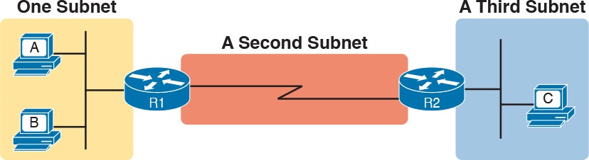
Figure 3: PC A and B in One Subnet, and PC C in a Different Subnet
The idea that hosts on the same link must be in the same subnet is much like the postal/zip code concept. All mailing addresses in the same town use the same postal code.
Addresses in another town, whether relatively nearby or on the other side of the country, have a different postal code. The postal code gives the postal service a better ability to automatically sort the mail to deliver it to the right location. For the same general reasons, hosts on the same LAN are in the same subnet, and hosts in different LANs are in different subnets.
Note that the point-to-point WAN link in the figure also needs a subnet. Figure 3 shows Router R1 connected to the LAN subnet on the left and to a WAN subnet on the right. Router R2 connects to that same WAN subnet. To do so, both R1 and R2 will have IP addresses on their WAN interfaces, and the addresses will be in the same subnet. (An Ethernet over MPLS [EoMPLS] WAN link has the same IP addressing needs, with each of the two routers having an IP address in the same subnet.)
The Ethernet LANs in Figure 3 also show a slightly different style of drawing, using simple lines with no Ethernet switch. Drawings of Ethernet LANs when the details of the LAN switches do not matter simply show each device connected to the same line, as shown in Figure 3. (This kind of drawing mimics the original Ethernet cabling before switches and hubs existed.)
Finally, because the routers’ main job is to forward packets from one subnet to another, routers typically connect to multiple subnets. For example, in this case, Router R1 connects to one LAN subnet on the left and one WAN subnet on the right. To do so, R1 will be configured with two different IP addresses, one per interface. These addresses will be in different subnets, because the interfaces connect the router to different subnets.
Determining the Number of Subnets
To determine the number of subnets required, the engineer must think about the internetwork as documented and count the locations that need a subnet. To do so, the engineer requires access to network diagrams, VLAN configuration details, and details about WAN links. For the types of links discussed in this course, you should plan for one subnet for every:
- VLAN
- Point-to-point serial link
- Ethernet emulation WAN link (EoMPLS)
NOTE: WAN technologies like MPLS allow subnetting options other than one subnet per pair of routers on the WAN, but this course only uses WAN technologies that have one subnet for each point-to-point WAN connection between two routers.
For example, imagine that the network planner has only Figure 4 on which to base the subnet design.
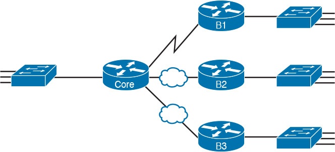
Figure 4: Four-Site Internetwork with Small Central Site
The number of subnets required cannot be fully predicted with only this figure. Certainly, three subnets will be needed for the WAN links, one per link. However, each LAN switch can be configured with a single VLAN, or with multiple VLANs. You can be certain that you need at least one subnet for the LAN at each site, but you might need more.
Next, consider the more detailed version of the same figure shown in Figure 5. In this case, the figure shows VLAN counts in addition to the same Layer 3 topology (the routers and the links connected to the routers). It also shows that the central site has many more switches, but the key fact on the left, regardless of how many switches exist, is that the central site has a total of 12 VLANs. Similarly, the figure lists each branch as having two VLANs. Along with the same three WAN subnets, this internetwork requires 21 subnets.

Figure 5: Four-Site Internetwork with Larger Central SiteFour-Site Internetwork with Larger Central Site
Finally, in a real job, you would consider the needs today as well as how much growth you expect in the internetwork over time. Any subnetting plan should include a reasonable estimate of the number of subnets you need to meet future needs.
Determining the Number of Hosts per Subnet
Determining the number of hosts per subnet requires knowing a few simple concepts and then doing a lot of research and questioning. Every device that connects to a subnet needs an IP address. For a totally new network, you can look at business plans—numbers of people at the site, devices on order, and so on—to get some idea of the possible devices. When expanding an existing network to add new sites, you can use existing sites as a point of comparison, and then find out which sites will get bigger or smaller. And don’t forget to count the router interface IP address in each subnet and the switch IP address used to remotely manage the switch.
Instead of gathering data for each and every site, planners often just use a few typical sites for planning purposes. For example, maybe you have some large sales offices and some small sales offices. You might dig in and learn a lot about only one large sales office and only one small sales office. Add that analysis to the fact that point-to-point links need a subnet with just two addresses, plus any analysis of more one-of-a-kind subnets, and you have enough information to plan the addressing and subnetting design.
For example, in Figure 6, the engineer has built a diagram that shows the number of hosts per LAN subnet in the largest branch, B1. For the two other branches, the engineer did not bother to dig to find out the number of required hosts. As long as the number of required IP addresses at sites B2 and B3 stays below the estimate of 50, based on larger site B1, the engineer can plan for 50 hosts in each branch LAN subnet and have plenty of addresses per subnet.
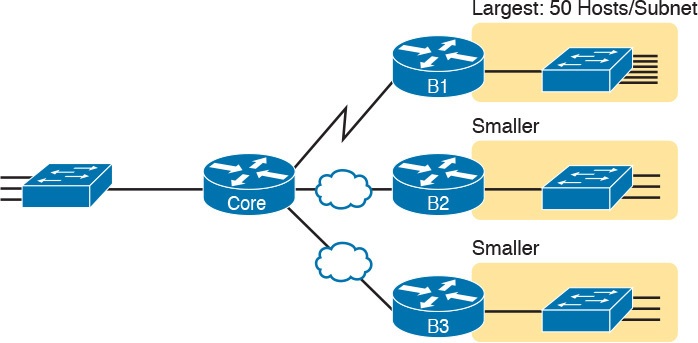
Figure 6: Large Branch B1 with 50 Hosts/Subnet
One Size Subnet Fits All—Or Not
The final choice in the initial planning step is to decide whether you will use a simpler design by using a one-size-subnet-fits-all philosophy. A subnet’s size, or length, is simply the number of usable IP addresses in the subnet. A subnetting design can either use one size subnet, or varied sizes of subnets, with pros and cons for each choice.
Defining the Size of a Subnet
Before you finish this course, you will learn all the details of how to determine the size of the subnet. For now, you just need to know a few specific facts about the size of subnets.
The engineer assigns each subnet a subnet mask, and that mask, among other things, defines the size of that subnet. The mask sets aside a number of host bits whose purpose is to number different host IP addresses in that subnet. Because you can number 2x things with x bits, if the mask defines H host bits, the subnet contains 2H – 2 unique numeric values.
However, the subnet’s size is not 2H. It’s 2H – 2, because two numbers in each subnet are reserved for other purposes. Each subnet reserves the numerically lowest value for the subnet number and the numerically highest value as the subnet broadcast address. As a result, the number of usable IP addresses per subnet is 2H – 2.
NOTE: The terms subnet number, subnet ID, and subnet address all refer to the number that represents or identifies a subnet.
Figure 7 shows the general concept behind the three-part structure of an IP address, focusing on the host part and the resulting subnet size.
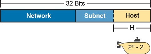
Figure 7: Subnet Size Concepts
One-Size Subnet Fits All
To choose to use a single-size subnet in an enterprise network, you must use the same mask for all subnets, because the mask defines the size of the subnet. But which mask?
One requirement to consider when choosing that one mask is this: That one mask must provide enough host IP addresses to support the largest subnet. To do so, the number of host bits (H) defined by the mask must be large enough so that 2H – 2 is larger than (or equal to) the number of host IP addresses required in the largest subnet.
For example, consider Figure 8. It shows the required number of hosts per LAN subnet. (The figure ignores the subnets on the WAN links, which require only two IP addresses each.) The branch LAN subnets require only 50 host addresses, but the main site LAN subnet requires 200 host addresses. To accommodate the largest subnet, you need at least 8 host bits. Seven host bits would not be enough, because 27 – 2 = 126. Eight host bits would be enough, because 28 – 2 = 254, which is more than enough to support 200 hosts in a subnet.
Figure 8: Network Using One Subnet Size
What’s the big advantage when using a single-size subnet? Operational simplicity. In other words, keeping it simple. Everyone on the IT staff who has to work with networking can get used to working with one mask—and one mask only. They will be able to answer all subnetting questions more easily, because everyone gets used to doing subnetting math with that one mask.
The big disadvantage for using a single-size subnet is that it wastes IP addresses. For example, in Figure 8, all the branch LAN subnets support 254 addresses, while the largest branch subnet needs only 50 addresses. The WAN subnets only need two IP addresses, but each supports 254 addresses, again wasting more IP addresses.
The wasted IP addresses do not actually cause a problem in most cases, however. Most organizations use private IP networks in their enterprise internetworks, and a single Class A or Class B private network can supply plenty of IP addresses, even with the waste.
Multiple Subnet Sizes (Variable-Length Subnet Masks)
To create multiple sizes of subnets in one Class A, B, or C network, the engineer must create some subnets using one mask, some with another, and so on. Different masks mean different numbers of host bits, and a different number of hosts in some subnets based on the 2H – 2 formula.
For example, consider the requirements listed earlier in Figure 8. It showed one LAN subnet on the left that needs 200 host addresses, three branch subnets that need 50 addresses, and three WAN links that need two addresses. To meet those needs, but waste fewer IP addresses, three subnet masks could be used, creating subnets of three different sizes, as shown in Figure 9.
Figure 9: Three Masks, Three Subnet Sizes
The smaller subnets now waste fewer IP addresses compared to the design shown earlier in Figure 8. The subnets on the right that need 50 IP addresses have subnets with 6 host bits, for 26 – 2 = 62 available addresses per subnet. The WAN links use masks with 2 host bits, for 22 – 2 = 2 available addresses per subnet.
However, some are still wasted, because you cannot set the size of the subnet as some arbitrary size. All subnets will be a size based on the 2H – 2 formula, with H being the number of host bits defined by the mask for each subnet.
One-Size Subnet Fits All (Mostly)
For the most part, this course explains subnetting using designs that use a single mask, creating a single subnet size for all subnets. Why? First, it makes the process of learning subnetting easier. Second, some types of analysis that you can do about a network—specifically, calculating the number of subnets in the classful network—only make sense when a single mask is used.
However, you still need to be ready to work with variable-length subnet masks (VLSM), which is the practice of using different masks for different subnets in the same classful IP network. However, all the examples and discussion up until that lesson purposefully avoid VLSM just to keep the discussion simpler, for the sake of learning to walk before you run.
Make Design Choices
Now that you know how to analyze the IP addressing and subnetting needs, the next major step examines how to apply the rules of IP addressing and subnetting to those needs and make some choices. In other words, now that you know how many subnets you need and how many host addresses you need in the largest subnet, how do you create a useful subnetting design that meets those requirements? The short answer is that you need to do the three tasks shown on the right side of Figure 10.
Figure 10: Input to the Design Phase, and Design Questions to Answer
Choose a Classful Network
In the original design for what we know of today as the Internet, companies used registered public classful IP networks when implementing TCP/IP inside the company. By the mid- 1990s, an alternative became more popular: private IP networks. This section discusses the background behind these two choices, because it impacts the choice of what IP network a company will then subnet and implement in its enterprise internetwork.
Public IP Networks
The original design of the Internet required that any company that connected to the Internet had to use a registered public IP network. To do so, the company would complete some paperwork, describing the enterprise’s internetwork and the number of hosts existing, plus plans for growth. After submitting the paperwork, the company would receive an assignment of either a Class A, B, or C network.
Public IP networks, and the administrative processes surrounding them, ensure that all the companies that connect to the Internet all use unique IP addresses. In particular, after a public IP network is assigned to a company, only that company should use the addresses in that network. That guarantee of uniqueness means that Internet routing can work well, because there are no duplicate public IP addresses.
For example, consider the example shown in Figure 11. Company 1 has been assigned public Class A network 1.0.0.0, and company 2 has been assigned public Class A network 2.0.0.0. Per the original intent for public addressing in the Internet, after these public network assignments have been made, no other companies can use addresses in Class A networks 1.0.0.0 or 2.0.0.0.
Figure 11: Two Companies with Unique Public IP Networks
This original address assignment process ensured unique IP addresses across the entire planet. The idea is much like the fact that your telephone number should be unique in the universe, your postal mailing address should also be unique, and your email address should also be unique. If someone calls you, your phone rings, but no one else’s phone rings. Similarly, if company 1 is assigned Class A network 1.0.0.0, and it assigns address 1.1.1.1 to a particular PC, that address should be unique in the universe. A packet sent through the Internet to destination 1.1.1.1 should only arrive at this one PC inside company 1, instead of being delivered to some other host.
Growth Exhausts the Public IP Address Space
By the early 1990s, the world was running out of public IP networks that could be assigned. During most of the 1990s, the number of hosts newly connected to the Internet was growing at a double-digit pace, per month. Companies kept following the rules, asking for public IP networks, and it was clear that the current address-assignment scheme could not continue without some changes. Simply put, the number of Class A, B, and C networks supported by the 32-bit address in IP version 4 (IPv4) was not enough to support one public classful network per organization, while also providing enough IP addresses in each company.
NOTE: The universe has run out of public IPv4 addresses in a couple of significant ways. IANA, which assigns public IPv4 address blocks to the five Regional Internet Registries (RIR) around the globe, assigned the last of the IPv4 address space in early 2011. By 2015, ARIN, the RIR for North America, exhausted its supply of IPv4 addresses, so that companies must return unused public IPv4 addresses to ARIN before they have more to assign to new companies. Try an online search for “ARIN depletion” to see pages about the current status of available IPv4 address space for just one RIR example.
The Internet community worked hard during the 1990s to solve this problem, coming up with several solutions, including the following:
- A new version of IP (IPv6), with much larger addresses (128 bit)
- Assigning a subset of a public IP network to each company, instead of an entire public IP network, to reduce waste
- Network Address Translation (NAT), which allows the use of private IP networks
These three solutions matter to real networks today. However, to stay focused on the topic of subnet design, this lesson focuses on the third option, and in particular, the private IP networks that can be used by an enterprise when also using NAT.
Focusing on the third item in the bullet list, NAT allows multiple companies to use the exact same private IP network, using the same IP addresses as other companies while still connecting to the Internet. For example, Figure 12 shows the same two companies connecting to the Internet as in Figure 11, but now with both using the same private Class A network 10.0.0.0.
Figure 12: Reusing the Same Private Network 10.0.0.0 with NAT
Both companies use the same classful IP network (10.0.0.0). Both companies can implement their subnet design internal to their respective enterprise internetworks, without discussing their plans. The two companies can even use the exact same IP addresses inside network 10.0.0.0. And amazingly, at the same time, both companies can even communicate with each other through the Internet.
The technology called Network Address Translation makes it possible for companies to reuse the same IP networks, as shown in Figure 12. NAT does this by translating the IP addresses inside the packets as they go from the enterprise to the Internet, using a small number of public IP addresses to support tens of thousands of private IP addresses. For now, accept that most companies use NAT, and therefore, they can use private IP networks for their internetworks.
Private IP Networks
Request For Comments (RFC) 1918 defines the set of private IP networks, as listed in Table 1. By definition, these private IP networks
- Will never be assigned to an organization as a public IP network
- Can be used by organizations that will use NAT when sending packets into the Internet
- Can also be used by organizations that never need to send packets into the Internet
So, when using NAT—and almost every organization that connects to the Internet uses NAT—the company can simply pick one or more of the private IP networks from the list of reserved private IP network numbers. RFC 1918 defines the list, which is summarized in Table 1.

Table 1: RFC 1918 Private Address Space
NOTE: According to an informal survey I ran on my blog a few years back, about half of the respondents said that their networks use private Class A network 10.0.0.0, as opposed to other private networks or public networks.
Choosing an IP Network During the Design Phase
Today, some organizations use private IP networks along with NAT, and some use public IP networks. Most new enterprise internetworks use private IP addresses throughout the network, along with NAT, as part of the connection to the Internet. Those organizations that already have registered public IP networks—often obtained before the addresses started running short in the early 1990s—can continue to use those public addresses throughout their enterprise networks.
After the choice to use a private IP network has been made, just pick one that has enough IP addresses. You can have a small internetwork and still choose to use private Class A network 10.0.0.0. It might seem wasteful to choose a Class A network that has over 16 million IP addresses, especially if you only need a few hundred. However, there’s no penalty or problem with using a private network that is too large for your current or future needs.
For the purposes of this course, most examples use private IP network numbers. For the design step to choose a network number, just choose a private Class A, B, or C network from the list of RFC 1918 private networks.
Regardless, from a math and concept perspective, the methods to subnet a public IP network versus a private IP network are the same.
Choose the Mask
If a design engineer followed the topics in this lesson so far, in order, he would know the following:
- The number of subnets required
- The number of hosts/subnet required
- That a choice was made to use only one mask for all subnets, so that all subnets are the same size (same number of hosts/subnet)
- The classful IP network number that will be subnetted
This section completes the design process, at least the parts described in this lesson, by discussing how to choose that one mask to use for all subnets. First, this section examines default masks, used when a network is not subnetted, as a point of comparison. Next, the concept of borrowing host bits to create subnet bits is explored. Finally, this section ends with an example of how to create a subnet mask based on the analysis of the requirements.
Classful IP Networks Before Subnetting
Before an engineer subnets a classful network, the network is a single group of addresses. In other words, the engineer has not yet subdivided the network into many smaller subsets called subnets.
When thinking about an unsubnetted classful network, the addresses in a network have only two parts: the network part and host part. Comparing any two addresses in the classful network:
The addresses have the same value in the network part.
The addresses have different values in the host part.
The actual sizes of the network and host part of the addresses in a network can be easily predicted, as shown in Figure 13.
Figure 13: Format of Unsubnetted Class A, B, and C Networks
In Figure 13, N and H represent the number of network and host bits, respectively. Class rules define the number of network octets (1, 2, or 3) for Classes A, B, and C, respectively; the figure shows these values as a number of bits. The number of host octets is 3, 2, or 1, respectively.
Continuing the analysis of classful network before subnetting, the number of addresses in one classful IP network can be calculated with the same 2H – 2 formula previously discussed. In particular, the size of an unsubnetted Class A, B, or C network is as follows:
- Class A: 224 – 2 = 16,777,214
- Class B: 216 – 2 = 65,534
- Class C: 28 – 2 = 254
Borrowing Host Bits to Create Subnet Bits
To subnet a network, the designer thinks about the network and host parts, as shown in Figure 13, and then the engineer adds a third part in the middle: the subnet part. However, the designer cannot change the size of the network part or the size of the entire address (32 bits). To create a subnet part of the address structure, the engineer borrows bits from the host part. Figure 14 shows the general idea.
Figure 14: Concept of Borrowing Host Bits
Figure 14 shows a rectangle that represents the subnet mask. N, representing the number of network bits, remains locked at 8, 16, or 24, depending on the class. Conceptually, the designer moves a (dashed) dividing line into the host field, with subnet bits (S) between the network and host parts, and the remaining host bits (H) on the right. The three parts must add up to 32, because IPv4 addresses consist of 32 bits.
Choosing Enough Subnet and Host Bits
The design process requires a choice of where to place the dashed line shown in Figure 14. But what is the right choice? How many subnet and host bits should the designer choose? The answers hinge on the requirements gathered in the early stages of the planning process:
- Number of subnets required
- Number of hosts/subnet
The bits in the subnet part create a way to uniquely number the different subnets that the design engineer wants to create. With 1 subnet bit, you can number 21 or 2 subnets. With 2 bits, 22 or 4 subnets, with 3 bits, 23 or 8 subnets, and so on. The number of subnet bits must be large enough to uniquely number all the subnets, as determined during the planning process.
At the same time, the remaining number of host bits must also be large enough to number the host IP addresses in the largest subnet. Remember, in this lesson, we assume the use of a single mask for all subnets. This single mask must support both the required number of subnets and the required number of hosts in the largest subnet. Figure 15 shows the concept.
Figure 15: Borrowing Enough Subnet and Host Bits
Figure 15 shows the idea of the designer choosing a number of subnet (S) and host (H) bits and then checking the math. 2S must be more than the number of required subnets, or the mask will not supply enough subnets in this IP network. Also, 2H – 2 must be more than the required number of hosts/subnet.
NOTE: The idea of calculating the number of subnets as 2S applies only in cases where a single mask is used for all subnets of a single classful network, as is being assumed in this lesson.
To effectively design masks, or to interpret masks that were chosen by someone else, you need a good working memory of the powers of 2. Use Numeric Reference Tables for your reference.
Example Design: 172.16.0.0, 200 Subnets, 200 Hosts
To help make sense of the theoretical discussion so far, consider an example that focuses on the design choice for the subnet mask. In this case, the planning and design choices so far tell us the following
- Use a single mask for all subnets.
- Plan for 200 subnets.
- Plan for 200 host IP addresses per subnet.
- Use private Class B network 172.16.0.0.
To choose the mask, the designer asks this question:
How many subnet (S) bits do I need to number 200 subnets?
From Table 2, you can see that S = 7 is not large enough (27 = 128), but S = 8 is enough (28 = 256). So, you need at least 8 subnet bits.
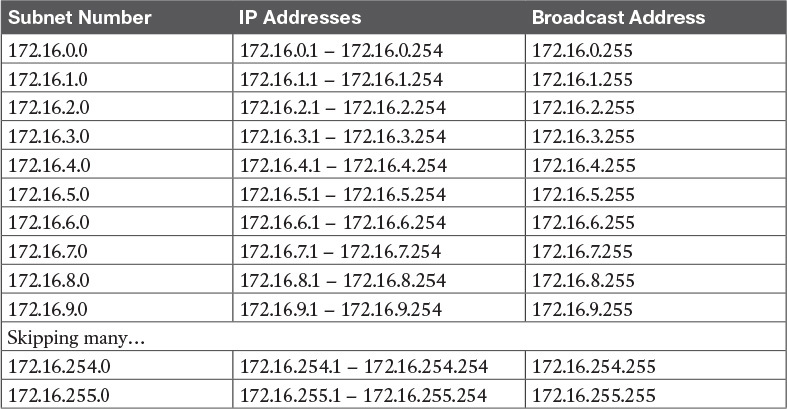
Table 2: First Ten Subnets, Plus the Last Few, from 172.16.0.0, 255.255.255.0
Next, the designer asks a similar question, based on the number of hosts per subnet:
How many host (H) bits do I need to number 200 hosts per subnet?
The math is basically the same, but the formula subtracts 2 when counting the number of hosts/subnet. From Table 2, you can see that H = 7 is not large enough (27 – 2 = 126), but H = 8 is enough (28 – 2 = 254).
Only one possible mask meets all the requirements in this case. First, the number of network bits (N) must be 16, because the design uses a Class B network. The requirements tell us that the mask needs at least 8 subnet bits, and at least 8 host bits. The mask only has 32 bits in it; Figure 16 shows the resulting mask.
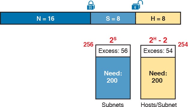
Figure 16: Example Mask Choice, N = 16, S = 8, H = 8
Masks and Mask Formats
Although engineers think about IP addresses in three parts when making design choices (network, subnet, and host), the subnet mask gives the engineer a way to communicate those design choices to all the devices in the subnet.
The subnet mask is a 32-bit binary number with a number of binary 1s on the left and with binary 0s on the right. By definition, the number of binary 0s equals the number of host bits; in fact, that is exactly how the mask communicates the idea of the size of the host part of the addresses in a subnet. The beginning bits in the mask equal binary 1, with those bit positions representing the combined network and subnet parts of the addresses in the subnet.
Because the network part always comes first, then the subnet part, and then the host part, the subnet mask, in binary form, cannot have interleaved 1s and 0s. Each subnet mask has one unbroken string of binary 1s on the left, with the rest of the bits as binary 0s.
After the engineer chooses the classful network and the number of subnet and host bits in a subnet, creating the binary subnet mask is easy. Just write down N 1s, S 1s, and then H 0s (assuming that N, S, and H represent the number of network, subnet, and host bits). Figure 17 shows the mask based on the previous example, which subnets a Class B network by creating 8 subnet bits, leaving 8 host bits.

Figure 17: Creating the Subnet Mask—Binary—Class B Network
In addition to the binary mask shown in Figure 17, masks can also be written in two other formats: the familiar dotted-decimal notation (DDN) seen in IP addresses and an even briefer prefix notation.
Build a List of All Subnets
This final task of the subnet design step determines the actual subnets that can be used, based on all the earlier choices. The earlier design work determined the Class A, B, or C network to use, and the (one) subnet mask to use that supplies enough subnets and enough host IP addresses per subnet. But what are those subnets? How do you identify or describe a subnet? This section answers these questions.
A subnet consists of a group of consecutive numbers. Most of these numbers can be used as IP addresses by hosts. However, each subnet reserves the first and last numbers in the group, and these two numbers cannot be used as IP addresses. In particular, each subnet contains the following:
Subnet number: Also called the subnet ID or subnet address, this number identifies the subnet. It is the numerically smallest number in the subnet. It cannot be used as an IP address by a host.
Subnet broadcast: Also called the subnet broadcast address or directed broadcast address, this is the last (numerically highest) number in the subnet. It also cannot be used as an IP address by a host.
IP addresses: All the numbers between the subnet ID and the subnet broadcast address can be used as a host IP address.
For example, consider the earlier case in which the design results were as follows:
- Network 172.16.0.0 (Class B)
- Mask 255.255.255.0 (for all subnets)
With some math, the facts about each subnet that exists in this Class B network can be calculated. In this case, Table 2 shows the first ten such subnets. It then skips many subnets and shows the last two (numerically largest) subnets.
After you have the network number and the mask, calculating the subnet IDs and other details for all subnets requires some math. In real life, most people use subnet calculators or subnet-planning tools.
Plan the Implementation
The next step, planning the implementation, is the last step before actually configuring the devices to create a subnet. The engineer first needs to choose where to use each subnet. For example, at a branch office in a particular city, which subnet from the subnet planning chart (Table 2) should be used for each VLAN at that site? Also, for any interfaces that require static IP addresses, which addresses should be used in each case? Finally, what range of IP addresses from inside each subnet should be configured in the DHCP server, to be dynamically leased to hosts for use as their IP address? Figure 18 summarizes the list of implementation planning tasks.

Figure 18: Facts Supplied to the Plan Implementation Step
Assigning Subnets to Different Locations
The job is simple: Look at your network diagram, identify each location that needs a subnet, and pick one from the table you made of all the possible subnets. Then, track it so that you know which ones you use where, using a spreadsheet or some other purpose-built subnet-planning tool. That’s it! Figure 19 shows a sample of a completed design using Table 2, which happens to match the initial design sample shown way back in Figure 1.
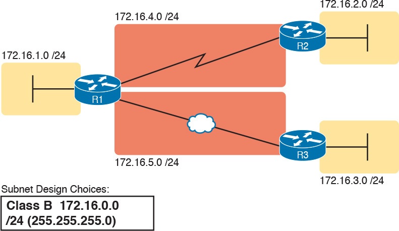
Figure 19: Example of Subnets Assigned to Different Locations
Although this design could have used any five subnets from Table 2, in real networks, engineers usually give more thought to some strategy for assigning subnets. For example, you might assign all LAN subnets lower numbers and WAN subnets higher numbers. Or you might slice off large ranges of subnets for different divisions of the company. Or you might follow that same strategy, but ignore organizational divisions in the company, paying more attention to geographies.
For example, for a U.S.-based company with a smaller presence in both Europe and Asia, you might plan to reserve ranges of subnets based on continent. This kind of choice is particularly useful when later trying to use a feature called route summarization.
Figure 20 shows the general benefit of placing addressing in the network for easier route summarization, using the same subnets from Table 2 again.
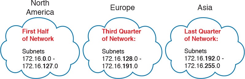
Figure 20: Reserving 50 Percent of Subnets for North America and 25 Percent Each for Europe and Asia
Choose Static and Dynamic Ranges per Subnet
Devices receive their IP address and mask assignment in one of two ways: dynamically by using Dynamic Host Configuration Protocol (DHCP) or statically through configuration. For DHCP to work, the network engineer must tell the DHCP server the subnets for which it must assign IP addresses. In addition, that configuration limits the DHCP server to only a subset of the addresses in the subnet. For static addresses, you simply configure the device to tell it what IP address and mask to use.
To keep things as simple as possible, most shops use a strategy to separate the static IP addresses on one end of each subnet, and the DHCP-assigned dynamic addresses on the other. It does not really matter whether the static addresses sit on the low end of the range of addresses or the high end.
For example, imagine that the engineer decides that, for the LAN subnets in Figure 19, the DHCP pool comes from the high end of the range, namely, addresses that end in .101 through .254. (The address that ends in .255 is, of course, reserved.) The engineer also assigns static addresses from the lower end, with addresses ending in .1 through .100. Figure 21 shows the idea.
Figure 21: Static from the Low End and DHCP from the High End
Figure 21 shows all three routers with statically assigned IP addresses that end in .1. The only other static IP address in the figure is assigned to the server on the left, with address 172.16.1.11 (abbreviated simply as .11 in the figure).
On the right, each LAN has two PCs that use DHCP to dynamically lease their IP addresses. DHCP servers often begin by leasing the addresses at the bottom of the range of addresses, so in each LAN, the hosts have leased addresses that end in .101 and .102, which are at the low end of the range chosen by design.

Troubleshooting Ethernet LANs
INTERNOLD NETWORKS CCNA LIVE WEBCLASS (INCLW)
Troubleshooting Ethernet LANs
Contents
Troubleshooting Ethernet LANs
This lesson focuses on the processes of verification and troubleshooting.
Verification refers to the process of confirming whether a network is working as designed.
Troubleshooting refers to the follow-on process that occurs when the network is not working as designed, by trying to determine the real reason why the network is not working correctly, so that it can be fixed.
Sometimes, when people take their first Cisco exam, they are surprised at the number of verification and troubleshooting questions. Each of these questions requires you to apply networking knowledge to unique problems, rather than just being ready to answer questions about lists of facts that you’ve memorized. You need to have skills beyond simply remembering a lot of facts.
This lesson discusses a wide number of topics.
- Analyzing switch interfaces and cabling
- Predicting where switches will forward frames
- Troubleshooting port security
- Analyzing VLANs and VLAN trunks
Perspectives on Applying Troubleshooting Methodologies
This first section of the lesson takes a brief diversion for one particular big idea: what troubleshooting processes could be used to resolve networking problems? Most CCNA Routing and Switching exam topics list the word “troubleshoot” along with some technology, mostly with some feature that you configure on a switch or router. One exam topic makes mention of the troubleshooting process. This first section examines the troubleshooting process as an end to itself.
The first important perspective on the troubleshooting process is this: you can troubleshoot using any process or method that you want. However, all good methods have the same characteristics that result in faster resolution of the problem, and a better chance of avoiding that same problem in the future.
The one exam topic that mentions troubleshooting methods uses some pretty common terminology found in troubleshooting methods both inside IT and in other industries as well.
The ideas make good common sense. From the exam topics:
- Step 1. Problem isolation and documentation: Problem isolation refers to the process of taking what you know about a possible issue, confirming that there is a problem, and determining which devices and cables could be part of the problem, and which ones are not part of the problem. This step also works best when the person troubleshooting the problem documents what they find, typically in a problem tracking system.
- Step 2. Resolve or escalate: Problem isolation should eventually uncover the root cause of the problem—that is, the cause which, if fixed, will resolve the problem. In short, resolving the problem means finding the root cause of the problem and fixing that problem. Of course, what do you do if you cannot find the root cause, or fix (resolve) that root cause once found? Escalate the problem. Most companies have a defined escalation process, with different levels of technical support and management support depending on whether the next step requires more technical expertise or management decision making.
- Step 3. Verify or monitor: You hear of a problem, you isolate the problem, document it, determine a possible root cause, and you try to resolve it. Now you need to verify that it really worked. In some cases, that may mean that you just do a few show commands. In other cases, you may need to keep an eye on it over a period of time, especially when you do not know what caused the root problem in the first place.
Like most real-life processes, the real troubleshooting process is seldom as neat as the three troubleshooting steps listed here.
You move between them, you attempt to resolve the problem, it may or may not work, you work through the process over and over, get help from the escalation team as needed, and so on. But following these kinds of steps can help you resolve problems more consistently, more quickly, especially when the team must get involved in troubleshooting a problem
Troubleshooting on the Exams
The exams ask you questions that not only assess your knowledge, but they assess your troubleshooting skills. To do that, the exam does not require you to follow any particular troubleshooting methods.
On the exam, you should focus on isolating the root cause of the problem, after which you will either (a) fix the problem or (b) answer a multichoice question about the symptoms and the root cause of the problem.
The exam uses two question types as the primary means to test troubleshooting skills. Sim questions begin with a broken configuration; your job is to find the configuration problem, and answer the question by fixing or completing the configuration. These are straightforward configuration troubleshooting questions, and you can recognize them on the exam when the exam tells you to answer the question by changing the configuration.
Simlet questions also give you a simulator where you access the command-line interface (CLI).
However, instead of changing the configuration, these questions require you to verify the current operation of the network and then answer multichoice questions about the current operation. These questions make you do the same kinds of commands you would use when doing problem isolation and documentation, and then assess what you found by asking you several multichoice questions.
At some point, whether you stop now or sometime when you have 10 to 15 spare minutes, take the time to search Cisco.com for “exam tutorial.” Cisco’s exam tutorial shows all the question types, including Sim and Simlet types, and you can take over the user interface to get a better sense for how to navigate in the same user interface you will see on exam day.
A Deeper Look at Problem Isolation
On the exam, you may do 5–10 show commands in a Simlet question before finding all the answers to all the multichoice questions within that one Simlet question. So it sometimes helps to go through problem isolation like what you would do in a real network.
In some questions, it may be obvious that the problem will be something to do with the switches or VLANs, but in others, you may have to do extra problem isolation work to even determine whether the problem is a WAN or LAN or routing problem, and which part of the network has the problem.
For example, consider the following problem based on the network in Figure 1. PC1 and PC2 supposedly sit in the same VLAN (10). At one time, the ping 10.1.1.2 command on PC1 worked; now it does not.
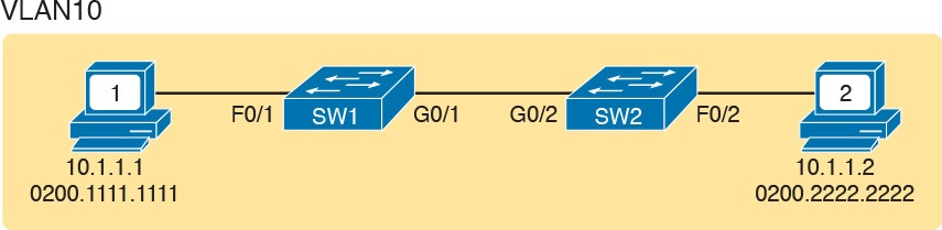
Figure 1: Network with a Ping Problem
NOTE: Ping command sends messages (inside IPv4 packets) that flow from one device to the other, and back, to test whether the IP network can deliver packets in both directions.
So, how do you attack this problem? If you doubt whether the figure is even correct, you could look at show command output to confirm the network topology. After it is confirmed, you could predict its normal working behavior based on your knowledge of LAN switching.
As a result, you could predict where a frame sent by PC1 to PC2 should flow. To isolate the problem, you could look in the switch MAC tables to confirm the interfaces out which the frame should be forwarded, possibly then finding that the interface connected to PC2 has failed.
This first problem showed a relatively small network, with only two networking devices (two Layer 2 switches). As a result, you would probably guess that the exam question focused on either interface issues or VLAN issues.
Other Simlet questions might instead begin with a larger network, but they might still require you to do problem isolation about the Ethernet topics. However, that problem isolation might need to start with Layer 3, just to decide where to begin looking for other problems.
For example, the user of PC1 in Figure 2 can usually connect to the web server on the right by entering www.example.com in PC1’s web browser. However, that web-browsing attempt fails right now. The user calls the help desk, and the problem is assigned to a network engineer to solve.
Figure 2: Layer 3 Problem Isolation
To begin the analysis, the network engineer can begin with the first tasks that would have to happen for a successful web-browsing session to occur.
For example, the engineer would try to confirm that PC1 can resolve the hostname (www.example.com) to the correct IP address used by the server on the right. At that point, the Layer 3 IP problem isolation process can proceed, to determine which of the six routing steps shown in the figure has failed.
The routing steps shown in Figure 2 are as follows:
- Step 1. PC1 sends the packet to its default gateway (R1) because the destination IP address (of the web server) is in a different subnet.
- Step 2. R1 forwards the packet to R2 based on R1’s routing table.
- Step 3. R2 forwards the packet to the web server based on R2’s routing table.
- Step 4. The web server sends a packet back toward PC1 based on the web server’s default gateway setting (R2).
- Step 5. R2 forwards the packet destined for PC1 by forwarding the packet to R1 according to R2’s routing table.
- Step 6. R1 forwards the packet to PC1 based on R1’s routing table.
Many engineers break down network problems as in this list, analyzing the Layer 3 path through the network, hop by hop, in both directions. This process helps you take the first attempt at problem isolation.
When the analysis shows which hop in the layer path fails, you can then look further at those details. And if in this case the Layer 3 problem isolation process discovers that Step 1, 3, 4, or 6 fails, the root cause might be related to Ethernet or other Layer 2 issues.
For example, imagine that the Layer 3 analysis determined that PC1 cannot even send a packet to its default gateway (R1), meaning that Step 1 in Figure 2 fails. To further isolate the problem and find the root causes, the engineer would need to determine the following:
- The MAC address of PC1 and of R1’s LAN interface
- The switch interfaces used on SW1 and SW2
- The interface status of each switch interface
- The VLANs that should be used
- The expected forwarding behavior of a frame sent by PC1 to R1 as the destination MAC address
By gathering and analyzing these facts, the engineer can most likely isolate the problem’s root cause and fix it.
Analyzing Switch Interface Status and Statistics
This section makes the transition from the process focus of the previous section to the first of four technology-focused sections of this lesson. That process begins with finding out whether each switch interface works, and if working, whether any statistics reveal any additional problems.
Unsurprisingly, Cisco switches do not use interfaces at all unless the interface is first considered to be in a functional or working state. In addition, the switch interface might be in a working state, but intermittent problems might still be occurring.
This section begins by looking at the Cisco switch interface status codes and what they mean so that you can know whether an interface is working. The rest of this section then looks at those more unusual cases in which the interface is working, but not working well, as revealed by different interface status codes and statistics.
Interface Status Codes and Reasons for Nonworking States
Cisco switches actually use two different sets of interface status codes—one set of two codes (words) that use the same conventions as do router interface status codes, and another set with a single code (word). Both sets of status codes can determine whether an interface is working.
The switch show interfaces and show interfaces description commands list the two-code status named the line status and protocol status. The line status generally refers to whether Layer 1 is working, with protocol status generally referring to whether Layer 2 is working.
NOTE: This section refers to these two status codes in shorthand by just listing the two codes with a slash between them, such as up/up.
The single-code interface status corresponds to different combinations of the traditional two-code interface status codes and can be easily correlated to those codes.
For example, the show interfaces status command lists a connected state for working interfaces, with the same meaning as the up/up state seen with the show interfaces and show interfaces description commands.
Table 1 lists the code combinations and some root causes that could have caused a particular interface status.
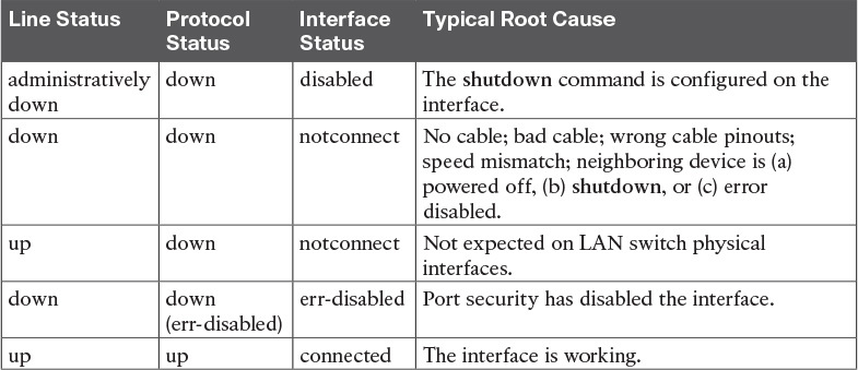
Table 1: LAN Switch Interface Status Codes
Examining the notconnect state for a moment, note that this state has many causes that have been mentioned through this section.
As you can see in the table, having a bad cable is just one of many reasons for the down/down state (or notconnect, per the show interfaces status command).
Some examples of the root causes of cabling problems include the following:
- The installation of any equipment that uses electricity, even non-IT equipment, can interfere with the transmission on the cabling, and make the link fail.
- The cable could be damaged, for example, if it lies under carpet. If the user’s chair keeps squashing the cable, eventually the electrical signal can degrade.
- Although optical cables do not suffer from electromagnetic interference (EMI), someone can try to be helpful and move a fiber-optic cable out of the way—bending it too much. A bend into too tight a shape can prevent the cable from transmitting bits (called macrobending).
For the other interface states listed in Table 1, only the up/up (connected) state needs more discussion. An interface can be in a working state, and it might really be working—or it might be working in a degraded state.
The next few topics discuss how to examine an up/up (connected) interface to find out whether it is working well or having problems.
Interface Speed and Duplex Issues
Many unshielded twisted-pair (UTP)-based Ethernet interfaces support multiple speeds, either full or half duplex, and support IEEE standard autonegotiation.
These same interfaces can also be configured to use a specific speed using the speed {10 | 100 | 1000} interface subcommand, and a specific duplex using the duplex {half | full} interface subcommand.
With both configured, a switch or router disables the IEEE-standard autonegotiation process on that interface.
The show interfaces and show interfaces status commands list both the actual speed and duplex settings on an interface, as demonstrated in Example 1.
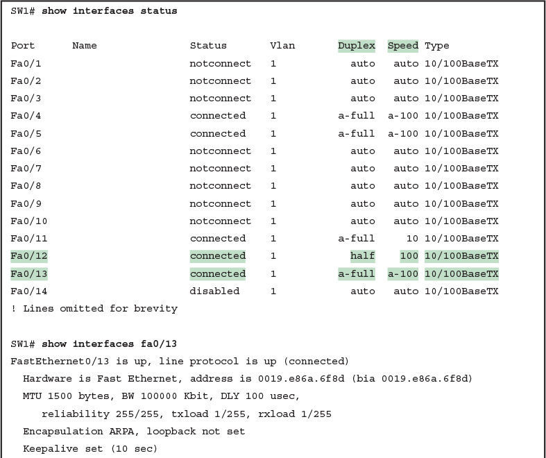
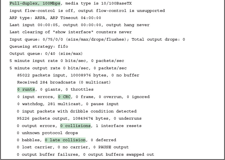
Example 1: Displaying Speed and Duplex Settings on Switch Interfaces
Although both commands in the example can be useful, only the show interfaces status command implies how the switch determined the speed and duplex settings. The command output lists autonegotiated settings with a prefix of a-.
For example, a-full means full duplex as autonegotiated, whereas full means full duplex but as manually configured. The example shades the command output that implies that the switch’s Fa0/12 interface’s speed and duplex were not found through autonegotiation, but Fa0/13 did use autonegotiation.
Note that the show interfaces fa0/13 command (without the status option) simply lists the speed and duplex for interface Fast Ethernet 0/13, with nothing implying that the values were learned through autonegotiation.
When the IEEE autonegotiation process works on both devices, both devices agree to the fastest speed supported by both devices. In addition, the devices use full duplex if it is supported by both devices, or half duplex if it is not. However, when one device has disabled autonegotiation, and the other device uses autonegotiation, the device using autonegotiation chooses the default duplex setting based on the current speed.
The defaults are as follows:
- If the speed is not known through any means, use 10 Mbps, half duplex.
- If the switch successfully senses the speed without IEEE autonegotiation, by just looking at the signal on the cable:
- If the speed is 10 or 100 Mbps, default to use half duplex.
- If the speed is 1,000 Mbps, default to use full duplex.
NOTE: Ethernet interfaces using speeds faster than 1 Gbps always use full duplex.
While autonegotiation works well, these defaults allow for the possibility of a difficult-to-troubleshoot problem called a duplex mismatch.
The “Autonegotiation” section in previous lesson explains how both devices could use the same speed, so the devices would consider the link to be up, but one side would use half-duplex and the other side would use full duplex.
The next example shows a specific case that causes a duplex mismatch.
In Figure 3, imagine that SW2’s Gi0/2 interface was configured with the speed 100 and duplex full commands (these settings are not recommended on a Gigabit-capable interface, by the way).
On Cisco switches, configuring both the speed and duplex commands disables IEEE autonegotiation on that port. If SW1’s Gi0/1 interface tries to use autonegotiation, SW1 would also use a speed of 100 Mbps, but default to use half duplex. Example 2 shows the results of this specific case on SW1.
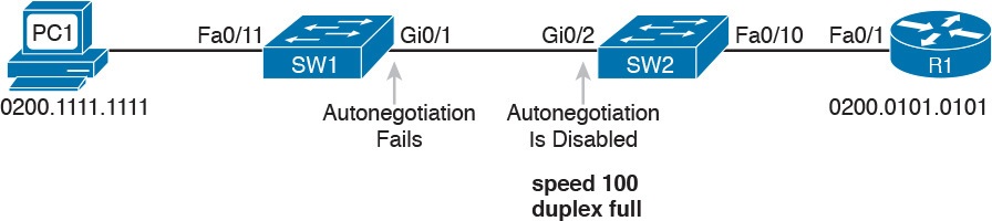
Figure 3: Conditions to Create a Duplex Mismatch Between SW1 and SW2

Example 2: Confirming Duplex Mismatch on Switch SW1
First, focusing on the command output, the command confirms SW1’s speed and duplex. It also lists a prefix of a- in the output, implying autonegotiation. Even with SW1 using autonegotiation defaults, the command still notes the values as being learned through autonegotiation.
Finding a duplex mismatch can be much more difficult than finding a speed mismatch, because if the duplex settings do not match on the ends of an Ethernet segment, the switch interface will still be in a connected (up/up) state. In this case, the interface works, but it might work poorly, with poor performance, and with symptoms of intermittent problems.
The reason is that the device using half-duplex uses carrier sense multiple access collision detect (CSMA/CD) logic, waiting to send when receiving a frame, believing collisions occur when they physically do not—and actually stopping sending a frame because the switch thinks a collision occurred. With enough traffic load, the interface could be in a connect state, but it’s extremely inefficient for passing traffic.
To identify duplex mismatch problems, check the duplex setting on each end of the link and watch for incrementing collision and late collision counters, as explained in the next section.
Common Layer 1 Problems on Working Interfaces
When the interface reaches the connect (up/up) state, the switch considers the interface to be working. The switch, of course, tries to use the interface, and at the same time, the switch keeps various interface counters.
These interface counters can help identify problems that can occur even though the interface is in a connect state. This section explains some of the related concepts and a few of the most common problems.
Whenever the physical transmission has problems, the receiving device might receive a frame whose bits have changed values.
These frames do not pass the error detection logic as implemented in the FCS field in the Ethernet trailer.
The receiving device discards the frame and counts it as some kind of input error. Cisco switches list this error as a CRC error, as highlighted in Example 3. (Cyclic redundancy check [CRC] is a term related to how the frame check sequence [FCS] math detects an error.)

Example 3: Interface Counters for Layer 1 Problems
The number of input errors, and the number of CRC errors, are just a few of the counters in the output of the show interfaces command. The challenge is to decide which counters you need to think about, which ones show that a problem is happening, and which ones are normal and of no concern.
The example highlights several of the counters as examples so that you can start to understand which ones point to problems and which ones are just counting normal events that are not problems. The following list shows a short description of each highlighted counter, in the order shown in the example:
- Runts: Frames that did not meet the minimum frame size requirement (64 bytes, including the 18-byte destination MAC, source MAC, type, and FCS). Can be caused by collisions.
- Giants: Frames that exceed the maximum frame size requirement (1518 bytes, including the 18-byte destination MAC, source MAC, type, and FCS).
- Input Errors: A total of many counters, including runts, giants, no buffer, CRC, frame, overrun, and ignored counts.
- CRC: Received frames that did not pass the FCS math; can be caused by collisions.
- Frame: Received frames that have an illegal format, for example, ending with a partial byte; can be caused by collisions.
- Packets Output: Total number of packets (frames) forwarded out the interface.
- Output Errors: Total number of packets (frames) that the switch port tried to transmit, but for which some problem occurred.
- Collisions: Counter of all collisions that occur when the interface is transmitting a frame.
- Late Collisions: The subset of all collisions that happen after the 64th byte of the frame has been transmitted. (In a properly working Ethernet LAN, collisions should occur within the first 64 bytes; late collisions today often point to a duplex mismatch.)
Note that many of these counters occur as part of the CSMA/CD process used when half duplex is enabled. Collisions occur as a normal part of the half-duplex logic imposed by CSMA/CD, so a switch interface with an increasing collisions counter might not even have a problem.
However, one problem, called late collisions, points to the classic duplex mismatch problem.
If a LAN design follows cabling guidelines, all collisions should occur by the end of the 64th byte of any frame. When a switch has already sent 64 bytes of a frame, and the switch receives a frame on that same interface, the switch senses a collision.
In this case, the collision is a late collision, and the switch increments the late collision counter in addition to the usual CSMA/CD actions to send a jam signal, wait a random time, and try again.
With a duplex mismatch, like the mismatch between SW1 and SW2 in Figure 3, the half-duplex interface will likely see the late collisions counter increment.
Why? The half-duplex interface sends a frame (SW1), but the full duplex neighbor (SW2) sends at any time, even after the 64th byte of the frame sent by the half-duplex switch.
So, just keep repeating the show interfaces command, and if you see the late collisions counter incrementing on a half-duplex interface, you might have a duplex mismatch problem.
A working interface (in an up/up state) can still suffer from issues related to the physical cabling as well. The cabling problems might not be bad enough to cause a complete failure, but the transmission failures result in some frames failing to pass successfully over the cable.
For example, excessive interference on the cable can cause the various input error counters to keep growing larger, especially the CRC counter. In particular, if the CRC errors grow, but the collisions counters do not, the problem might simply be interference on the cable. (The switch counts each collided frame as one form of input error as well.)
Predicting Where Switches Will Forward Frames
Predicting the Contents of the MAC Address Table
Switches learn MAC addresses and then use the entries in the MAC address table to make a forwarding/filtering decision for each frame.
To know exactly how a particular switch will forward an Ethernet frame, you need to examine the MAC address table on a Cisco switch.
The more formal troubleshooting process begins with a mental process where you predict where frames should flow in the LAN. As an exercise, review Figure 4 and try to create a MAC address table on paper for each switch. Include the MAC addresses for both PCs, as well as the Gi0/1 MAC address for R1. (Assume that all three are assigned to VLAN 10.) Then predict which interfaces would be used to forward a frame sent by Fred, Barney, and R1 to every other device.
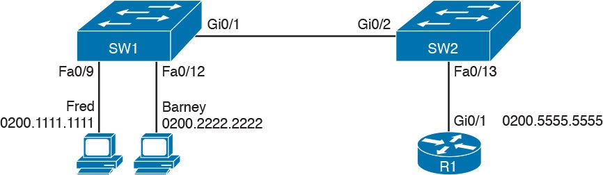
Sample Network Used in Switch MAC Learning Examples
The MAC table entries you predict in this case define where you think frames will flow. Even though this sample network in Figure 4 shows only one physical path through the Ethernet LAN, the exercise should be worthwhile, because it forces you to correlate what you’d expect to see in the MAC address table with how the switches forward frames. Figure 5 shows the resulting MAC table entries for PCs Fred and Barney, as well as for Router R1.
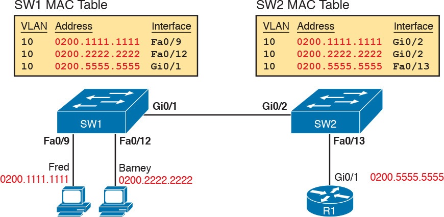
Predictions for MAC Table Entries on SW1 and SW2
While Figure 5 shows the concepts, Example 4 lists the same facts but in the form of the show mac address-table dynamic command on the switches. This command lists all dynamically learned MAC table entries on a switch, for all VLANs.
Example 4 Examining SW1 and SW2 Dynamic MAC Address Table Entries
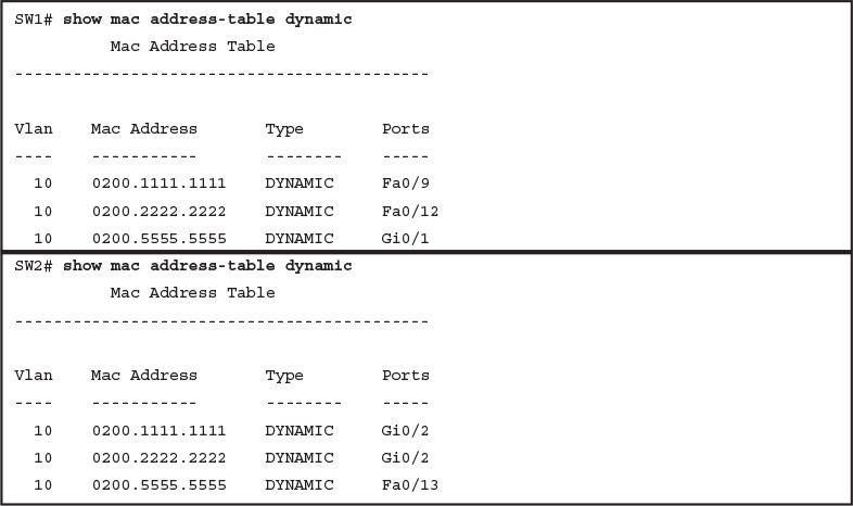
Examining SW1 and SW2 Dynamic MAC Address Table Entries
When predicting the MAC address table entries, you need to imagine a frame sent by a device to another device on the other side of the LAN and then determine which switch ports the frame would enter as it passes through the LAN. For example, if Barney sends a frame to Router R1, the frame would enter SW1’s Fa0/12 interface, so SW1 has a MAC table entry that lists Barney’s 0200.2222.2222 MAC address with Fa0/12. SW1 would forward Barney’s frame to SW2, arriving on SW2’s Gi0/2 interface, so SW2’s MAC table lists Barney’s MAC address (0200.2222.2222) with interface Gi0/2.
After you predict the expected contents of the MAC address tables, you can then examine what is actually happening on the switches, as described in the next section.
Analyzing the Forwarding Path
Troubleshooting revolves around three big ideas: predicting what should happen, determining what is happening that is different than what should happen, and figuring out why that different behavior is happening. This next section discusses how to look at what is actually happening in a VLAN based on those MAC address tables, first using a summary of switch forwarding logic and then showing an example.
The following list summarizes switch forwarding logic including the LAN switching features discussed in this study:
Step 1. Process functions on the incoming interface, if the interface is currently in an up/up (connected) state, as follows:
A. If configured, apply port security logic to filter the frame as appropriate.
B. If the port is an access port, determine the interface’s access VLAN.
C. If the port is a trunk, determine the frame’s tagged VLAN.
Step 2. Make a forwarding decision. Look for the frame’s destination MAC address in the MAC address table, but only for entries in the VLAN identified in Step 1. If the destination MAC is...
A. Found (unicast), forward the frame out the only interface listed in the matched address table entry.
B. Not found (unicast), flood the frame out all other access ports (except the incoming port) in that same VLAN, plus out trunks that have not restricted the VLAN from that trunk.
C. Broadcast, flood the frame, with the same rules as the previous step.
For an example of this process, consider a frame sent by Barney to its default gateway, R1 (0200.5555.5555). Using the steps just listed, the following occurs:
Step 1. Input interface processing:
A. The port does not happen to have port security enabled.
B. SW1 receives the frame on its Fa0/12 interface, an access port in VLAN 10.
Step 2. Make a forwarding decision: SW1 looks in its MAC address table for entries in VLAN 10:
A. SW1 finds an entry (known unicast) for 0200.5555.5555, associated with VLAN 10, outgoing interface Gi0/1, so SW1 forwards the frame only out interface Gi0/1. (This link is a VLAN trunk, so SW1 adds a VLAN 10 tag to the 802.1Q trunking header.)
At this point, the frame with source 0200.2222.2222 (Barney) and destination 0200.5555.5555 (R1) is on its way to SW2. You can then apply the same logic for SW2, as follows:
Step 1. Input interface processing:
A. The port does not happen to have port security enabled.
B. SW2 receives the frame on its Gi0/2 interface, a trunk; the frame lists a tag of VLAN 10. (SW2 will remove the 802.1Q header as well.)
Step 2. Make a forwarding decision: SW2 looks for its MAC table for entries in VLAN 10:
A. SW2 finds an entry (known unicast) for 0200.5555.5555, associated with VLAN 10, outgoing interface Fa0/13, so SW2 forwards the frame only out interface Fa0/13.
At this point, the frame should be on its way, over the Ethernet cable between SW2 and R1.
Analyzing Port Security Operations on an Interface
Generally speaking, any analysis of the forwarding process should consider any security features that might discard some frames or packets. For example, both routers and switches can be configured with access control lists (ACL) that examine the packets and frames being sent or received on an interface, with the router or switch discarding those packets/frames.
This study does not include coverage of switch ACLs, but the exams do cover a switch feature called port security. Port security feature can be used to cause the switch to discard some frames sent into and out of an interface. Port security has three basic features with which it determines which frames to filter:
Limit which specific MAC addresses can send and receive frames on a switch interface, discarding frames to/from other MAC addresses
Limit the number of MAC addresses using the interface, discarding frames to/from MAC addresses learned after the maximum limit is reached
A combination of the previous two points
The first port security troubleshooting step should be to find which interfaces have port security enabled, followed by a determination as to whether any violations are currently occurring. The trickiest part relates to the differences in what the IOS does in reaction to violations based on the switchport port-security violation violation-mode interface subcommand, which tells the switch what to do when a violation occurs. The general process to find port security issues is as follows:
Step 1. Identify all interfaces on which port security is enabled (show running-config or show port-security).
Step 2. Determine whether a security violation is currently occurring based in part on the violation mode of the interface’s port security configuration, as follows:
A. shutdown: The interface will be in an err-disabled state, and the port security port status will be secure-down.
B. restrict: The interface will be in a connected state, the port security port status will be secure-up, but the show port-security interface command will show an incrementing violations counter.
C. protect: The interface will be in a connected state, and the show port-security interface command will not show an incrementing violations counter.
Step 3. In all cases, compare the port security configuration to the diagram and to the Last Source Address field in the output of the show port-security interface command.
Because IOS reacts so differently with shutdown mode as compared to restrict and protect modes, the next few pages explain the differences—first for shutdown mode, then for the other two modes.
Troubleshooting Shutdown Mode and Err-disabled Recovery
Troubleshooting Step 2A refers to the interface err-disabled (error-disabled) state. This state verifies that the interface has been configured to use port security, that a violation has occurred, and that no traffic is allowed on the interface at the present time. This interface state implies that the shutdown violation mode is used, because it is the only one of the three port security modes that causes the interface to be disabled.
To recover from an err-disabled state, the interface must be shut down with the shutdown command, and then enabled with the no shutdown command. Example 5 lists an example in which the interface is in an err-disabled state.
Example 5 Using Port Security to Define Correct MAC Addresses of Particular Interfaces
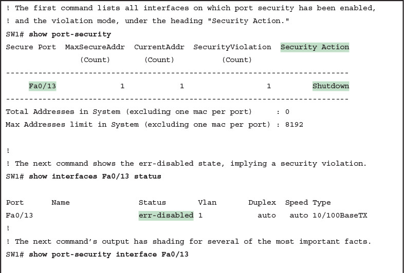
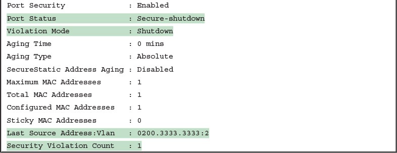
The output of the show port-security interface command lists a couple of items helpful in the troubleshooting process. The port status of secure-shutdown means that the interface is disabled for all traffic as a result of a violation while in port security shutdown mode; this state is not used by the protect and restrict modes. The port security port status of secure-shutdown also means that the interface state should be err-disabled.
Note that in shutdown mode, the violations counter (at the bottom of the output) does not keep incrementing. Basically, once the first violating frame triggers IOS to move the port to an err-disabled state, IOS ignores any other incoming frames (not even counting them) until the engineer uses the shutdown and no shutdown commands on the interface, in succession. Note that the process of recovering the interface also resets the violation counter back to 0. Finally, note that the second-to-last line lists the source MAC address of the last frame received on the interface. This value can prove useful in identifying the MAC address of the device that caused the violation.
Figure 6 summarizes these behaviors, assuming the same scenario shown in the example.
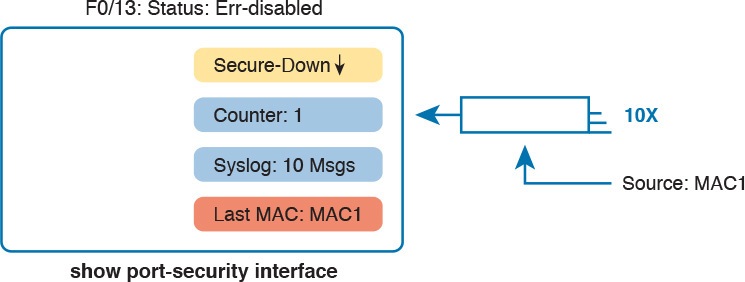
Summary of Actions: Port Security Violation Mode Shutdown
Troubleshooting Restrict and Protect Modes
The restrict and protect violation modes take a much different approach to securing ports. These modes still discard offending traffic, but the interface remains in a connected (up/up) state, and in a port security state of secure-up. As a result, the port continues to forward good traffic and discard offending traffic.
Having a port in a seemingly good state that also discards traffic can be a challenge when troubleshooting. Basically, you have to know about this possible pitfall, and then know how to tell when port security is discarding some traffic on a port even though the interface status looks good.
The show port-security interface command reveals whether protect mode has discarded frames using the “last source address” item in the output. Example 6 shows a sample configuration and show command when using protect mode. In this case, the port is configured to allow Fa0/13 to receive frames sent by 0200.1111.1111 only. Ten frames have arrived, with a variety of source MAC addresses, with the last frame’s source MAC address being 0200.3333.3333.
Example 6 Port Security Using Protect Mode
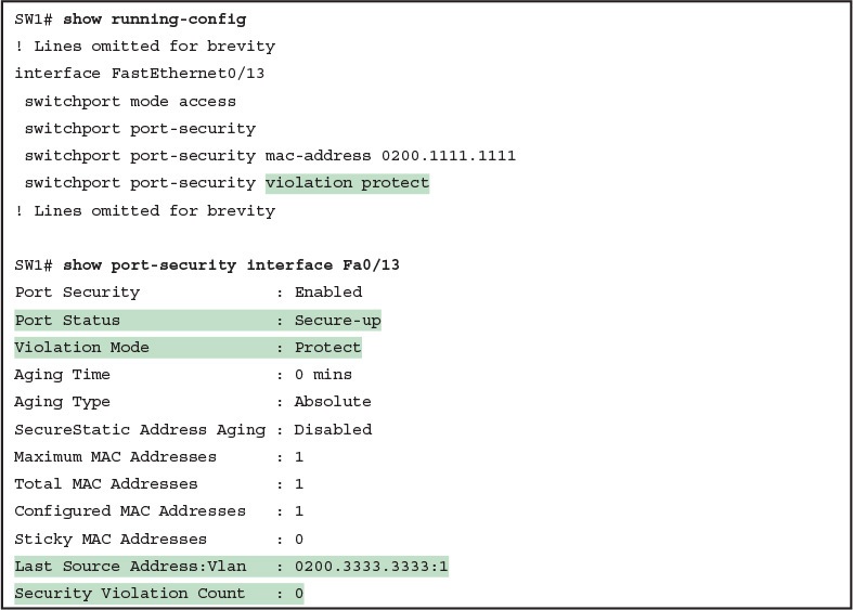
Port Security Using Protect Mode
In protect mode, the show port-security interface command reveals practically nothing about whether the interfaces happen to be discarding traffic or not. For instance, in this case, this show command output was gathered after many frames had been sent by a PC with MAC address 0200.3333.3333, with all the frames being discarded by the switch because of port security. The command output shows the disallowed PC’s 0200.3333.3333 MAC address as the last source MAC address in a received frame. However, if another frame with an allowed MAC address arrived (in this case, source MAC 0200.1111.1111), the next instance of the show command would list 0200.1111.1111 as the last source address. In particular, note that the interface remains in a secure-up state, and the violation counter does not increment.
Figure 7 summarizes the key points about the operation of Port Security protect mode, assuming a mix of frames with different source addresses. The figure emphasizes unpredictability of the last source MAC listed in the output, and the fact that the counter does not increment and that no syslog messages are generated for violating frames.
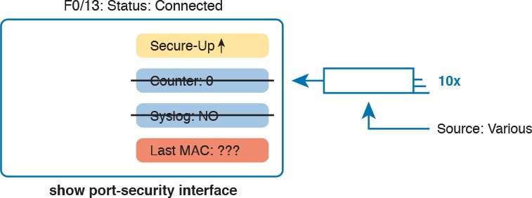
Summary of Actions: Port Security Violation Mode Protect
If this example had used violation mode restrict instead of protect, the port status would have also remained in a secure-up state; however, IOS would show some indication of port security activity, such as the incrementing violation counter as well as syslog messages. Example 7 shows an example of the violation counter and ends with an example port security syslog message. In this case, 97 incoming frames so far violated the rules, with the most recent frame having a source MAC address of 0200.3333.3333.
Example 7 Port Security Using Violation Mode Restrict
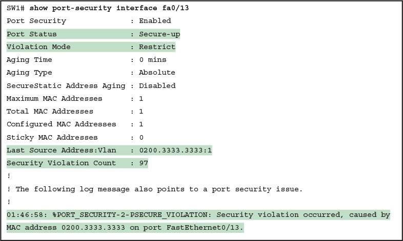
Port Security Using Violation Mode Restrict
Figure 8 summarizes the key points about the restrict mode for port security. In this case, the figure matches the same scenario as the example again, with 97 total violating frames arriving so far, with the most recent being from source MAC MAC3.
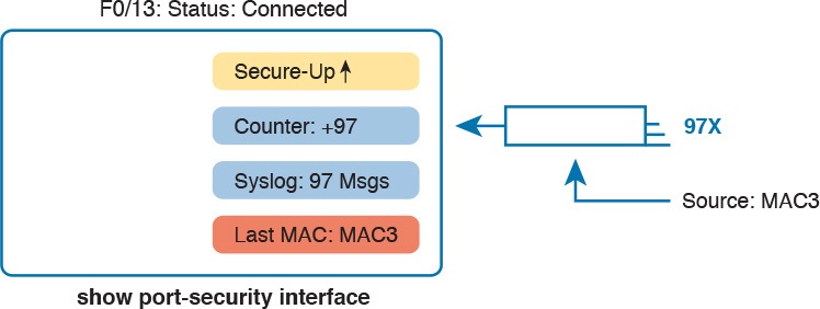
Summary of Actions: Port Security Violation Mode Restrict
For the exams, a port security violation might not be a problem; it might be the exact function intended. The question text might well explicitly state what port security should be doing. In these cases, it can be quicker to just immediately look at the port security configuration. Then, compare the configuration to the MAC addresses of the devices connected to the interface. The most likely problem on the exams is that the MAC addresses have been misconfigured or that the maximum number of MAC addresses has been set too low.
Analyzing VLANs and VLAN Trunks
A switch’s forwarding process, as discussed earlier in the section “Analyzing the Forwarding Path,” depends in part on VLANs and VLAN trunking. Before a switch can forward frames in a particular VLAN, the switch must know about a VLAN and the VLAN must be active. And before a switch can forward a frame over a VLAN trunk, the trunk must currently allow that VLAN to pass over the trunk. This final of the five major sections in this lesson focuses on VLAN and VLAN trunking issues, specifically issues that impact the frame switching process. The four potential issues are as follows:
Step 1. Identify all access interfaces and their assigned access VLANs and reassign into the correct VLANs as needed.
Step 2. Determine whether the VLANs both exist (configured or learned with VTP) and are active on each switch. If not, configure and activate the VLANs to resolve problems as needed.
Step 3. Check the allowed VLAN lists, on the switches on both ends of the trunk, and ensure that the lists of allowed VLANs are the same.
Step 4. Check for incorrect configuration settings that result in one switch operating as a trunk, with the neighboring switch not operating as a trunk.
Ensuring That the Right Access Interfaces Are in the Right VLANs
To ensure that each access interface has been assigned to the correct VLAN, engineers simply need to determine which switch interfaces are access interfaces instead of trunk interfaces, determine the assigned access VLANs on each interface, and compare the information to the documentation. The show commands listed in Table 2 can be particularly helpful in this process.
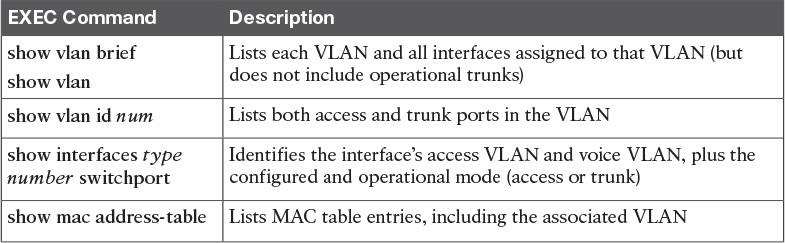
Commands That Can Find Access Ports and VLANs
If possible, start this step with the show vlan and show vlan brief commands, because they list all the known VLANs and the access interfaces assigned to each VLAN. Be aware, however, that these two commands do not list operational trunks. The output does list all other interfaces (those not currently trunking), no matter whether the interface is in a working or nonworking state.
If the show vlan and show interface switchport commands are not available in a particular exam question, the show mac address-table command can also help identify the access VLAN. This command lists the MAC address table, with each entry including a MAC address, interface, and VLAN ID. If the exam question implies that a switch interface connects to a single device PC, you should only see one MAC table entry that lists that particular access interface; the VLAN ID listed for that same entry identifies the access VLAN. (You cannot make such assumptions for trunking interfaces.)
After you determine the access interfaces and associated VLANs, if the interface is assigned to the wrong VLAN, use the switchport access vlan vlan-id interface subcommand to assign the correct VLAN ID.
Access VLANs Not Being Defined
Switches do not forward frames for VLANs that are (a) not configured or (b) configured but disabled (shut down). This section summarizes the best ways to confirm that a switch knows that a particular VLAN exists, and if it exists, determines the state of the VLAN.
First, on the issue of whether a VLAN is defined, a VLAN can be defined to a switch in two ways: using the vlan number global configuration command, or it can be learned from another switch using VTP. This study purposefully ignores VTP as much as possible, so for this discussion, consider that the only way for a switch to know about a VLAN is to have a vlan command configured on the local switch.
Next, the show vlan command always lists all VLANs known to the switch, but the show running-config command does not. Switches configured as VTP servers and clients do not list the vlan commands in the running-config nor the startup-config file; on these switches, you must use the show vlan command. Switches configured to use VTP transparent mode, or that disable VTP, list the vlan configuration commands in the configuration files. (Use the show vtp status command to learn the current VTP mode of a switch.)
After you determine that a VLAN does not exist, the problem might be that the VLAN simply needs to be defined.
Access VLANs Being Disabled
For any existing VLANs, also verify whether the VLAN is active. The show vlan command should list one of two VLAN state values, depending on the current state: either active or act/lshut. The second of these states means that the VLAN is shut down. Shutting down a VLAN disables the VLAN on that switch only, so that the switch will not forward frames in that VLAN.
Switch IOS gives you two similar configuration methods with which to disable (shutdown) and enable (no shutdown) a VLAN. Example 8 shows how, first by using the global command [no] shutdown vlan number and then using the VLAN mode subcommand [no] shutdown. The example shows the global commands enabling and disabling VLANs 10 and 20, respectively, and using VLAN subcommands to enable and disable VLANs 30 and 40 (respectively).
Example 8 Enabling and Disabling VLANs on a Switch
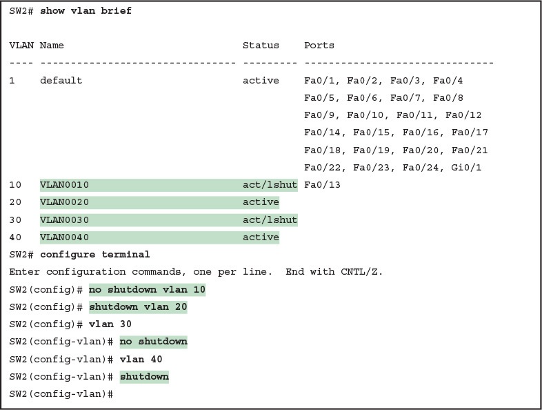
Enabling and Disabling VLANs on a Switch
Mismatched Trunking Operational States
Trunking can be configured correctly so that both switches forward frames for the same set of VLANs. However, trunks can also be misconfigured, with a couple of different results. In some cases, both switches conclude that their interfaces do not trunk. In other cases, one switch believes that its interface is correctly trunking, while the other switch does not.
The most common incorrect configuration—which results in both switches not trunking—is a configuration that uses the switchport mode dynamic auto command on both switches on the link. The word “auto” just makes us all want to think that the link would trunk automatically, but this command is both automatic and passive. As a result, both switches passively wait on the other device on the link to begin negotiations.
With this particular incorrect configuration, the show interfaces switchport command on both switches confirms both the administrative state (auto), as well as the fact that both switches operate as “static access” ports. Example 9 highlights those parts of the output from this command.
Example 9 Operational Trunking State
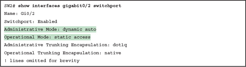
Operational Trunking State
A different incorrect trunking configuration results in one switch with an operational state of “trunk,” while the other switch has an operational state of “static access.” When this combination of events happens, the interface works a little. The status on each end will be up/up or connected. Traffic in the native VLAN will actually cross the link successfully. However, traffic in all the rest of the VLANs will not cross the link.
Figure 9 shows the incorrect configuration along with which side trunks and which does not. The side that trunks (SW1 in this case) enables trunking always, using the command switchport mode trunk. However, this command does not disable DTP negotiations. To cause this particular problem, SW1 also disables DTP negotiation using the switchport nonegotiate command. SW2’s configuration also helps create the problem, by using a trunking option that relies on DTP. Because SW1 has disabled DTP, SW2’s DTP negotiations fail, and SW2 does not trunk.
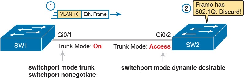
Mismatched Trunking Operational States
In this case, SW1 treats its G0/1 interface as a trunk, and SW2 treats its G0/2 interface as an access port (not a trunk). As shown in the figure at Step 1, SW1 could (for example) forward a frame in VLAN 10 (Step 1). However, SW2 would view any frame that arrives with an 802.1Q header as illegal, because SW2 treats its G0/2 port as an access port. So, SW2 discards any 802.1Q frames received on that port.
To deal with the possibility of this problem, always check the trunk’s operational state on both sides of the trunk. The best commands to check trunking-related facts are show interfaces trunk and show interfaces switchport.
NOTE: Frankly, in real life, just avoid this kind of configuration. However, the switches do not prevent you from making these types of mistakes, so you need to be ready.

Implementing Ethernet Virtual LANs
INTERNOLD NETWORKS CCNA LIVE WEBCLASS (INCLW)
Implementing Ethernet Virtual LANs
Contents
Implementing Ethernet Virtual LANs
At their heart, Ethernet switches receive Ethernet frames, make decisions, and then forward (switch) those Ethernet frames. That core logic revolves around MAC addresses, the interface in which the frame arrives, and the interfaces out which the switch forwards the frame.
Several switch features have some impact on an individual switch’s decisions about where to forward frames, virtual LANs (VLAN) easily have the biggest impact on those choices.
This lesson examines the concepts and configuration of VLANs.
The first major section of the lesson explains the core concepts. These concepts include how VLANs work on a single switch, how to use VLAN trunking to create VLANs that span across multiple switches, and how to forward traffic between VLANs using a router.
The second major section shows how to configure VLANs and VLAN trunks: how to statically assign interfaces to a VLAN.
Virtual LAN Concepts
Before understanding VLANs, you must first have a specific understanding of the definition of a LAN. For example, from one perspective, a LAN includes all the user devices, servers, switches, routers, cables, and wireless access points in one location. However, an alternative narrower definition of a LAN can help in understanding the concept of a virtual LAN:
A LAN includes all devices in the same broadcast domain.
A broadcast domain includes the set of all LAN-connected devices, so that when any of the devices sends a broadcast frame, all the other devices get a copy of the frame. So, from one perspective, you can think of a LAN and a broadcast domain as being basically the same thing.
Without VLANs, a switch considers all its interfaces to be in the same broadcast domain. That is, for one switch, when a broadcast frame entered one switch port, the switch forwarded that broadcast frame out all other ports. With that logic, to create two different LAN broadcast domains, you had to buy two different Ethernet LAN switches, as shown in Figure 1.

Figure 1: Creating Two Broadcast Domains with Two Physical Switches and No VLANs
With support for VLANs, a single switch can accomplish the same goals of the design in Figure 1—to create two broadcast domains—with a single switch. With VLANs, a switch can configure some interfaces into one broadcast domain and some into another, creating multiple broadcast domains. These individual broadcast domains created by the switch are called virtual LANs (VLAN).
For example, in Figure 2, the single switch creates two VLANs, treating the ports in each VLAN as being completely separate. The switch would never forward a frame sent by Dino (in VLAN 1) over to either Wilma or Betty (in VLAN 2).

Figure 2: Creating Two Broadcast Domains Using One Switch and VLANs
Designing campus LANs to use more VLANs, each with a smaller number of devices, often helps improve the LAN in many ways. For example, a broadcast sent by one host in a VLAN will be received and processed by all the other hosts in the VLAN—but not by hosts in a different VLAN. Limiting the number of hosts that receive a single broadcast frame reduces the number of hosts that waste effort processing unneeded broadcasts. It also reduces security risks, because fewer hosts see frames sent by any one host. These are just a few reasons for separating hosts into different VLANs. The following list summarizes the most common reasons for choosing to create smaller broadcast domains (VLANs):
To reduce CPU overhead on each device by reducing the number of devices that receive each broadcast frame
To reduce security risks by reducing the number of hosts that receive copies of frames that the switches flood (broadcasts, multicasts, and unknown unicasts)
To improve security for hosts that send sensitive data by keeping those hosts on a separate VLAN
To create more flexible designs that group users by department, or by groups that work together, instead of by physical location
To solve problems more quickly, because the failure domain for many problems is the same set of devices as those in the same broadcast domain
To reduce the workload for the Spanning Tree Protocol (STP) by limiting a VLAN to a single access switch
This lesson does not examine all the reasons for VLANs in more depth. However, know that most enterprise networks use VLANs quite a bit. The rest of this lesson looks closely at the mechanics of how VLANs work across multiple Cisco switches, including the required configuration. To that end, the next section examines VLAN trunking, a feature required when installing a VLAN that exists on more than one LAN switch.
Creating Multiswitch VLANs Using Trunking
Configuring VLANs on a single switch requires only a little effort: You simply configure each port to tell it the VLAN number to which the port belongs. With multiple switches, you have to consider additional concepts about how to forward traffic between the switches.
When using VLANs in networks that have multiple interconnected switches, the switches need to use VLAN trunking on the links between the switches. VLAN trunking causes the switches to use a process called VLAN tagging, by which the sending switch adds another header to the frame before sending it over the trunk. This extra trunking header includes a VLAN identifier (VLAN ID) field so that the sending switch can associate the frame with a particular VLAN ID, and the receiving switch can then know in what VLAN each frame belongs.
Figure 3 shows an example that demonstrates VLANs that exist on multiple switches, but it does not use trunking. First, the design uses two VLANs: VLAN 10 and VLAN 20. Each switch has two ports assigned to each VLAN, so each VLAN exists in both switches. To forward traffic in VLAN 10 between the two switches, the design includes a link between switches, with that link fully inside VLAN 10. Likewise, to support VLAN 20 traffic between switches, the design uses a second link between switches, with that link inside VLAN 20
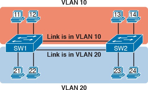
Figure 3: Multiswitch VLAN Without VLAN Trunking
VLAN Tagging Concepts
VLAN trunking creates one link between switches that supports as many VLANs as you need. As a VLAN trunk, the switches treat the link as if it were a part of all the VLANs. At the same time, the trunk keeps the VLAN traffic separate, so frames in VLAN 10 would not go to devices in VLAN 20, and vice versa, because each frame is identified by VLAN number as it crosses the trunk. Figure 4 shows the idea, with a single physical link between the two switches.
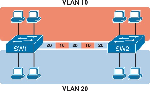
Figure 4: Multiswitch VLAN with Trunking
The use of trunking allows switches to pass frames from multiple VLANs over a single physical connection by adding a small header to the Ethernet frame. For example, Figure 5 shows PC11 sending a broadcast frame on interface Fa0/1 at Step 1. To flood the frame, switch SW1 needs to forward the broadcast frame to switch SW2. However, SW1 needs to let SW2 know that the frame is part of VLAN 10, so that after the frame is received, SW2 will flood the frame only into VLAN 10, and not into VLAN 20. So, as shown at Step 2, before sending the frame, SW1 adds a VLAN header to the original Ethernet frame, with the VLAN header listing a VLAN ID of 10 in this case.
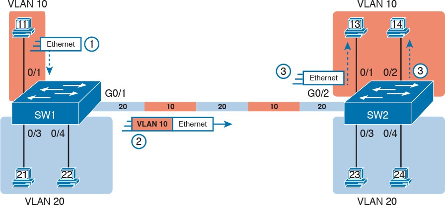
Figure 5: VLAN Trunking Between Two Switches
When SW2 receives the frame, it understands that the frame is in VLAN 10. SW2 then removes the VLAN header, forwarding the original frame out its interfaces in VLAN 10 (Step 3).
For another example, consider the case when PC21 (in VLAN 20) sends a broadcast. SW1 sends the broadcast out port Fa0/4 (because that port is in VLAN 20) and out Gi0/1 (because it is a trunk, meaning that it supports multiple different VLANs). SW1 adds a trunking header to the frame, listing a VLAN ID of 20. SW2 strips off the trunking header after determining that the frame is part of VLAN 20, so SW2 knows to forward the frame out only ports Fa0/3 and Fa0/4, because they are in VLAN 20, and not out ports Fa0/1 and Fa0/2, because they are in VLAN 10.
The 802.1Q and ISL VLAN Trunking Protocols
Cisco has supported two different trunking protocols over the years: Inter-Switch Link (ISL) and IEEE 802.1Q. Cisco created the ISL long before 802.1Q, in part because the IEEE had not yet defined a VLAN trunking standard. Years later, the IEEE completed work on the 802.1Q standard, which defines a different way to do trunking. Today, 802.1Q has become the more popular trunking protocol, with Cisco not even supporting ISL in some of its newer models of LAN switches, including the 2960 switches.
While both ISL and 802.1Q tag each frame with the VLAN ID, the details differ. 802.1Q inserts an extra 4-byte 802.1Q VLAN header into the original frame’s Ethernet header, as shown at the top of Figure 6. As for the fields in the 802.1Q header, only the 12-bit VLAN ID field inside the 802.1Q header matters. This 12-bit field supports a theoretical maximum of 212 (4096) VLANs, but in practice it supports a maximum of 4094. (Both 802.1Q and ISL use 12 bits to tag the VLAN ID, with two reserved values [0 and 4095].)
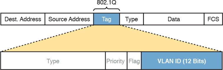
Fgiure 6: 802.1Q Trunking
Cisco switches break the range of VLAN IDs (1–4094) into two ranges: the normal range and the extended range. All switches can use normal-range VLANs with values from 1 to 1005. Only some switches can use extended-range VLANs with VLAN IDs from 1006 to 4094. The rules for which switches can use extended-range VLANs depend on the configuration of the VLAN Trunking Protocol (VTP), which is discussed briefly in the section “VLAN Trunking Configuration,” later in this lesson.
802.1Q also defines one special VLAN ID on each trunk as the native VLAN (defaulting to use VLAN 1). By definition, 802.1Q simply does not add an 802.1Q header to frames in the native VLAN. When the switch on the other side of the trunk receives a frame that does not have an 802.1Q header, the receiving switch knows that the frame is part of the native VLAN. Note that because of this behavior, both switches must agree on which VLAN is the native VLAN.
The 802.1Q native VLAN provides some interesting functions, mainly to support connections to devices that do not understand trunking. For example, a Cisco switch could be cabled to a switch that does not understand 802.1Q trunking. The Cisco switch could send frames in the native VLAN—meaning that the frame has no trunking header—so that the other switch would understand the frame. The native VLAN concept gives switches the capability of at least passing traffic in one VLAN (the native VLAN), which can allow some basic functions, like reachability to telnet into a switch.
Forwarding Data Between VLANs
If you create a campus LAN that contains many VLANs, you typically still need all devices to be able to send data to all other devices. This next topic discusses some concepts about how to route data between those VLANs.
First, it helps to know a few terms about some categories of LAN switches. All the Ethernet switch functions described so far use the details and logic defined by OSI Layer 2 protocols. For example, Chapter 7, “Analyzing Ethernet LAN Switching,” discussed how LAN switches receive Ethernet frames (a Layer 2 concept), look at the destination Ethernet MAC address (a Layer 2 address), and forward the Ethernet frame out some other interface. This lesson has already discussed the concept of VLANs as broadcast domains, which is yet another Layer 2 concept.
While some LAN switches work just as described so far, some LAN switches have even more functions. LAN switches that forward data based on Layer 2 logic, often go by the name Layer 2 switch. However, some other switches can do some functions like a router, using additional logic defined by Layer 3 protocols. These switches go by the name multilayer switch, or Layer 3 switch. This section first discusses how to forward data between VLANs when using Layer 2 switches and ends with a brief discussion of how to use Layer 3 switches.
Routing Packets Between VLANs with a Router
When including VLANs in a campus LAN design, the devices in a VLAN need to be in the same subnet. Following the same design logic, devices in different VLANs need to be in different subnets. For example, in Figure 7, the two PCs on the left sit in VLAN 10, in subnet 10. The two PCs on the right sit in a different VLAN (20), with a different subnet (20).

Figure 7: Layer 2 Switch Does Not Route Between the VLANs
NOTE:The figure refers to subnets somewhat generally, like “subnet 10,” just so the subnet numbers do not distract. Also, note that the subnet numbers do not have to be the same number as the VLAN numbers.
Figure 7 shows the switch as if it were two switches broken in two to emphasize the point that Layer 2 switches will not forward data between two VLANs. When configured with some ports in VLAN 10 and others in VLAN 20, the switch acts like two separate switches in which it will forward traffic. In fact, one goal of VLANs is to separate traffic in one VLAN from another, preventing frames in one VLAN from leaking over to other VLANs. For example, when Dino (in VLAN 10) sends any Ethernet frame, if SW1 is a Layer 2 switch, that switch will not forward the frame to the PCs on the right in VLAN 20.
The network as a whole needs to support traffic flowing into and out of each VLAN, even though the Layer 2 switch does not forward frames outside a VLAN. The job of forwarding data into and out of a VLAN falls to routers. Instead of switching Layer 2 Ethernet frames between the two VLANs, the network must route Layer 3 packets between the two subnets.
That previous paragraph has some very specific wording related to Layers 2 and 3, so take a moment to reread and reconsider it for a moment. The Layer 2 logic does not let the Layer 2 switch forward the Layer 2 protocol data unit (L2PDU), the Ethernet frame, between VLANs. However, routers can route Layer 3 PDUs (L3PDU) (packets) between subnets as their normal job in life.
For example, Figure 8 shows a router that can route packets between subnets 10 and 20. The figure shows the same Layer 2 switch as shown in Figure 7, with the same perspective of the switch being split into parts with two different VLANs, and with the same PCs in the same VLANs and subnets. Now Router R1 has one LAN physical interface connected to the switch and assigned to VLAN 10, and a second physical interface connected to the switch and assigned to VLAN 20. With an interface connected to each subnet, the Layer 2 switch can keep doing its job—forwarding frames inside a VLAN, while the router can do its job—routing IP packets between the subnets.
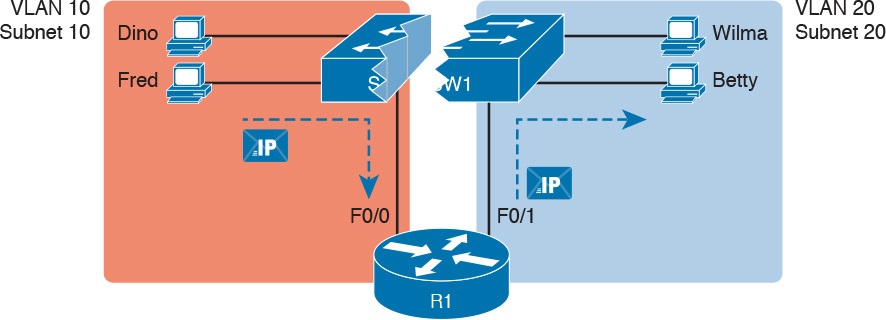
Figure 8: Routing Between Two VLANs on Two Physical Interfaces
The figure shows an IP packet being routed from Fred, which sits in one VLAN/subnet, to Betty, which sits in the other. The Layer 2 switch forwards two different Layer 2 Ethernet frames: one in VLAN 10, from Fred to R1’s F0/0 interface, and the other in VLAN 20, from R1’s F0/1 interface to Betty. From a Layer 3 perspective, Fred sends the IP packet to its default router (R1), and R1 routes the packet out another interface (F0/1) into another subnet where Betty resides.
While the design shown in Figure 8 works, it uses too many physical interfaces, one per VLAN. A much less expensive (and much preferred) option uses a VLAN trunk between the switch and router, requiring only one physical link between the router and switch, while supporting all VLANs. Trunking can work between any two devices that choose to support it: between two switches, between a router and a switch, or even between server hardware and a switch.
Figure 9 shows the same design idea as Figure 8, with the same packet being sent from Fred to Betty, except now R1 uses VLAN trunking instead of a separate link for each VLAN.
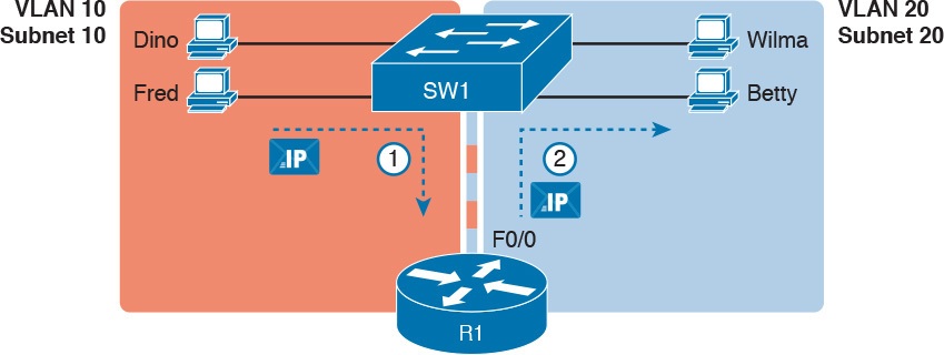
Figure 9: Routing Between Two VLANs Using a Trunk on the Router
NOTE: Because the router has a single physical link connected to the LAN switch, this design is sometimes called a router-on-a-stick
As a brief aside about terminology, many people describe the concept in Figures 11-8 and 11-9 as “routing packets between VLANs.” You can use that phrase, and people know what you mean. However, note that this phrase is not literally true, because it refers to routing packets (a Layer 3 concept) and VLANs (a Layer 2 concept). It just takes fewer words to say something like “routing between VLANs” rather than the literally true but long “routing Layer 3 packets between Layer 3 subnets, with those subnets each mapping to a Layer 2 VLAN.”
Routing Packets Between VLANs with a Router
Routing packets using a physical router, even with the VLAN trunk in the router-on-a-stick model shown in Figure 9, still has one significant problem: performance. The physical link puts an upper limit on how many bits can be routed, and less expensive routers tend to be less powerful, and might not be able to route a large enough number of packets per second (pps) to keep up with the traffic volumes.
The ultimate solution moves the routing functions inside the LAN switch hardware. Vendors long ago started combining the hardware and software features of their Layer 2 LAN switches, plus their Layer 3 routers, creating products called Layer 3 switches (also known as multilayer switches). Layer 3 switches can be configured to act only as a Layer 2 switch, or they can be configured to do both Layer 2 switching as well as Layer 3 routing.
Today, many medium- to large-sized enterprise campus LANs use Layer 3 switches to route packets between subnets (VLANs) in a campus.
In concept, a Layer 3 switch works a lot like the original two devices on which the Layer 3 switch is based: a Layer 2 LAN switch and a Layer 3 router. In fact, if you take the concepts and packet flow shown in Figure 8, with a separate Layer 2 switch and Layer 3 router, and then imagine all those features happening inside one device, you have the general idea of what a Layer 3 switch does. Figure 10 shows that exact concept, repeating many details of Figure 8, but with an overlay that shows the one Layer 3 switch doing the Layer 2 switch functions and the separate Layer 3 routing function.
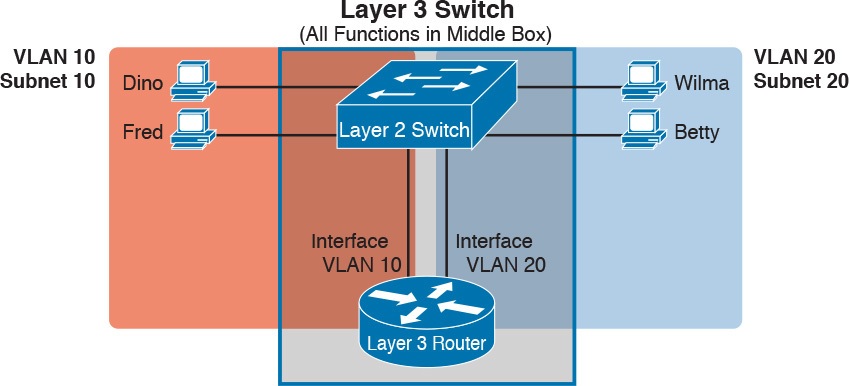
Figure 10: Multilayer Switch: Layer 2 Switching with Layer 3 Routing in One Device
This lesson introduces the core concepts of routing IP packets between VLANs (or more accurately, between the subnets on the VLANs). Chapter 18, “Configuring IPv4 Addresses and Static Routes,” shows how to configure designs that use an external router with router-on-a-stick. This lesson now turns its attention to configuration and verification tasks for VLANs and VLAN trunks.
VLAN and VLAN Trunking Configuration and Verification
Cisco switches do not require any configuration to work. You can purchase Cisco switches, install devices with the correct cabling, turn on the switches, and they work. You would never need to configure the switch, and it would work fine, even if you interconnected switches, until you needed more than one VLAN. But if you want to use VLANs—and most enterprise networks do—you need to add some configuration.
This lesson separates the VLAN configuration details into two major sections. The first section looks at how to configure access interfaces, which are switch interfaces that do not use VLAN trunking. The second part shows how to configure interfaces that do use VLAN trunking.
Creating VLANs and Assigning Access VLANs to an Interface
This section shows how to create a VLAN, give the VLAN a name, and assign interfaces to a VLAN. To focus on these basic details, this section shows examples using a single switch, so VLAN trunking is not needed.
For a Cisco switch to forward frames in a particular VLAN, the switch must be configured to believe that the VLAN exists. In addition, the switch must have nontrunking interfaces (called access interfaces) assigned to the VLAN, and/or trunks that support the VLAN. The configuration steps for access interfaces are as follows, with the trunk configuration shown later in the section “VLAN Trunking Configuration”:
Step 1. To configure a new VLAN, follow these steps:
A. From configuration mode, use the vlan vlan-id command in global configuration mode to create the VLAN and to move the user into VLAN configuration mode.
B. (Optional) Use the name name command in VLAN configuration mode to list a name for the VLAN. If not configured, the VLAN name is VLANZZZZ, where ZZZZ is the four-digit decimal VLAN ID.
Step 2. For each access interface (each interface that does not trunk, but instead belongs to a single VLAN), follow these steps:
A. Use the interface type number command in global configuration mode to move into interface configuration mode for each desired interface.
B. Use the switchport access vlan id-number command in interface configuration mode to specify the VLAN number associated with that interface.
C. (Optional) Use the switchport mode access command in interface configuration mode to make this port always operate in access mode (that is, to not trunk).
While the list might look a little daunting, the process on a single switch is actually pretty simple. For example, if you want to put the switch’s ports in three VLANs—11, 12, and 13—you just add three vlan commands: vlan 11, vlan 12, and vlan 13. Then, for each interface, add a switchport access vlan 11 (or 12 or 13) command to assign that interface to the proper VLAN.
NOTE: The term default VLAN (as shown in the exam topics) refers to the default setting on the switchport access vlan vlan-id command, and that default is VLAN ID 1. In other words, by default, each port is assigned to access VLAN 1.
VLAN Configuration Example 1: Full VLAN Configuration
Example 1 shows the configuration process of adding a new VLAN and assigning access interfaces to that VLAN. Figure 11 shows the network used in the example, with one LAN switch (SW1) and two hosts in each of three VLANs (1, 2, and 3). The example shows the details of the two-step process for VLAN 2 and the interfaces in VLAN 2, with the configuration of VLAN 3 deferred until the next example.
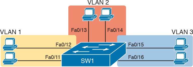
Figure 11: Network with One Switch and Three VLANs
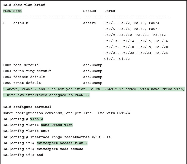
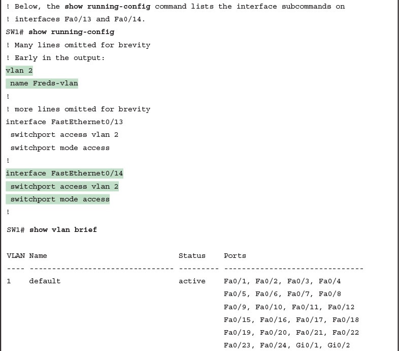
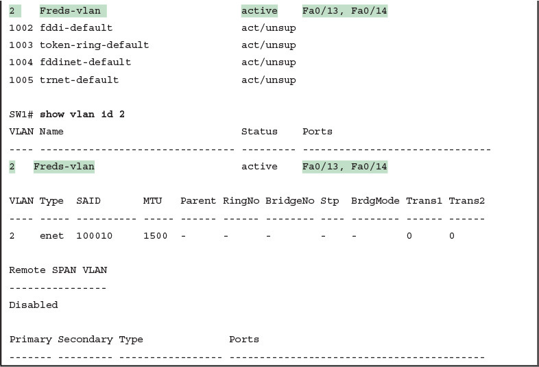
Example 1: Configuring VLANs and Assigning VLANs to Interfaces
The example begins with the show vlan brief command, confirming the default settings of five nondeletable VLANs, with all interfaces assigned to VLAN 1. (VLAN 1 cannot be deleted, but can be used. VLANs 1002–1005 cannot be deleted and cannot be used as access VLANs today.) In particular, note that this 2960 switch has 24 Fast Ethernet ports (Fa0/1–Fa0/24) and two Gigabit Ethernet ports (Gi0/1 and Gi0/2), all of which are listed as being in VLAN 1 per that first command’s output.
Next, the example shows the process of creating VLAN 2 and assigning interfaces Fa0/13 and Fa0/14 to VLAN 2. Note in particular that the example uses the interface range command, which causes the switchport access vlan 2 interface subcommand to be applied to both interfaces in the range, as confirmed in the show running-config command output at the end of the example.
After the configuration has been added, to list the new VLAN, the example repeats the show vlan brief command. Note that this command lists VLAN 2, name Freds-vlan, and the interfaces assigned to that VLAN (Fa0/13 and Fa0/14). The show vlan id 2 command that follows then confirms that ports Fa0/13 and Fa0/14 are assigned to VLAN 2.
The example surrounding Figure 11 uses six switch ports, all of which need to operate as access ports. That is, each port should not use trunking, but instead should be assigned to a single VLAN, as assigned by the switchport access vlan vlan-id command. However, as configured in Example 1, these interfaces could negotiate to later become trunk ports, because the switch defaults to allow the port to negotiate trunking and decide whether to act as an access interface or as a trunk interface.
For ports that should always act as access ports, add the optional interface subcommand switchport mode access. This command tells the switch to only allow the interface to be an access interface. The upcoming section “VLAN Trunking Configuration” discusses more details about the commands that allow a port to negotiate whether it should use trunking.
VLAN Configuration Example 2: Shorter VLAN Configuration
Example 1 shows several of the optional configuration commands, with a side effect of being a bit longer than is required. Example 2 shows a much briefer alternative configuration, picking up the story where Example 1 ended and showing the addition of VLAN 3 (as shown in Figure 11). Note that SW1 does not know about VLAN 3 at the beginning of this example.
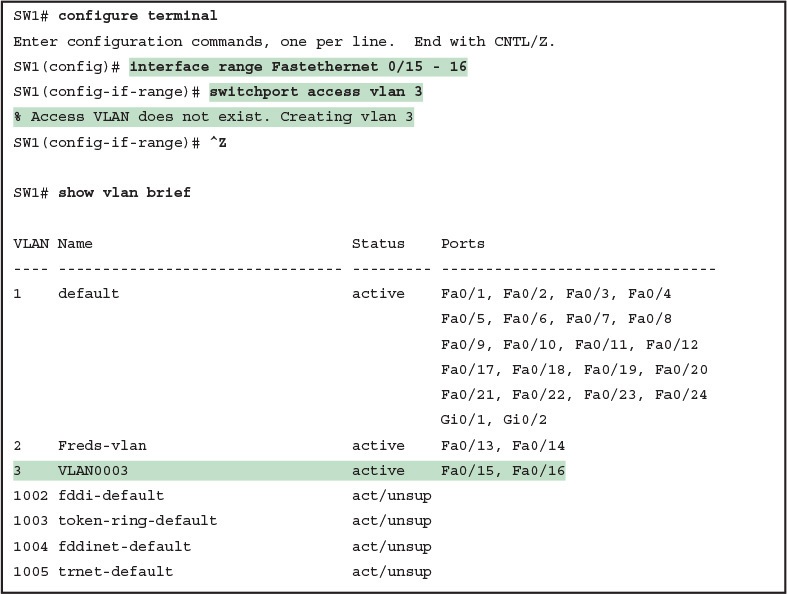
Example 2: Shorter VLAN Configuration Example (VLAN 3)
Example 2 shows how a switch can dynamically create a VLAN—the equivalent of the vlan vlan-id global config command—when the switchport access vlan interface subcommand refers to a currently unconfigured VLAN. This example begins with SW1 not knowing about VLAN 3. When the switchport access vlan 3 interface subcommand was used, the switch realized that VLAN 3 did not exist, and as noted in the shaded message in the example, the switch created VLAN 3, using a default name (VLAN0003). No other steps are required to create the VLAN. At the end of the process, VLAN 3 exists in the switch, and interfaces Fa0/15 and Fa0/16 are in VLAN 3, as noted in the shaded part of the show vlan brief command output.
VLAN Trunking Protocol
Before showing more configuration examples, you also need to know something about a Cisco protocol and tool called the VLAN Trunking Protocol (VTP). VTP is a Cisco proprietary tool on Cisco switches that advertises each VLAN configured in one switch (with the vlan number command) so that all the other switches in the campus learn about that VLAN. However, for various reasons, many enterprises choose not to use VTP.
However, VTP has some small impact on how every Cisco Catalyst switch works, even if you do not try to use VTP. This brief section introduces enough details of VTP so that you can see these small differences in VTP that cannot be avoided.
This study attempts to ignore VTP as much as is possible. To that end, all examples in this study use switches that have either been set to use VTP transparent mode (with the vtp mode transparent global command) or to disable it (with the vtp mode off global command). Both options allow the administrator to configure both standard- and extended-range VLANs, and the switch lists the vlan commands in the running-config file.
Finally, on a practical note, if you happen to do lab exercises with real switches or with simulators, and you see unusual results with VLANs, check the VTP status with the show vtp status command. If your switch uses VTP server or client mode, you will find:
The server switches can configure VLANs in the standard range only (1–1005).
The client switches cannot configure VLANs.
Both servers and clients may be learning new VLANs from other switches, and seeing their VLANs deleted by other switches, because of VTP.
The show running-config command does not list any vlan commands.
If possible in lab, switch to VTP transparent mode and ignore VTP for your switch configuration practice until you are ready to focus on how VTP works when studying for the ICND2 exam topics.
NOTE: Do not change VTP settings on any switch that also connects to the production network until you know how VTP works and you talk with experienced colleagues. If the switch you configure connects to other switches, which in turn connect to switches used in the production LAN, you could accidentally change the VLAN configuration in other switches with serious impact to the operation of the network. Be careful and never experiment with VTP settings on a switch unless it, and the other switches connected to it, have absolutely no physical links connected to the production LAN.
VLAN Trunking Configuration
Trunking configuration between two Cisco switches can be very simple if you just statically configure trunking. For example, if two Cisco 2960 switches connect to each other, they support only 802.1Q and not ISL. You could literally add one interface subcommand for the switch interface on each side of the link (switchport mode trunk), and you would create a VLAN trunk that supported all the VLANs known to each switch.
However, trunking configuration on Cisco switches includes many more options, including several options for dynamically negotiating various trunking settings. The configuration can either predefine different settings or tell the switch to negotiate the settings, as follows:
The type of trunking: IEEE 802.1Q, ISL, or negotiate which one to use
The administrative mode: Whether to always trunk, always not trunk, or negotiate
First, consider the type of trunking. Cisco switches that support ISL and 802.1Q can negotiate which type to use, using the Dynamic Trunking Protocol (DTP). If both switches support both protocols, they use ISL; otherwise, they use the protocol that both support. Today, many Cisco switches do not support the older ISL trunking protocol. Switches that support both types of trunking use the switchport trunk encapsulation {dot1q | isl | negotiate} interface subcommand to either configure the type or allow DTP to negotiate the type.
DTP can also negotiate whether the two devices on the link agree to trunk at all, as guided by the local switch port’s administrative mode. The administrative mode refers to the configuration setting for whether trunking should be used. Each interface also has an operational mode, which refers to what is currently happening on the interface, and might have been chosen by DTP’s negotiation with the other device. Cisco switches use the switchport mode interface subcommand to define the administrative trunking mode, as listed in Table 1.
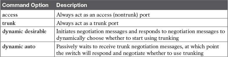
Table 1: Trunking Administrative Mode Options with the switchport mode Command
For example, consider the two switches shown in Figure 12. This figure shows an expansion of the network of Figure 11, with a trunk to a new switch (SW2) and with parts of VLANs 1 and 3 on ports attached to SW2. The two switches use a Gigabit Ethernet link for the trunk. In this case, the trunk does not dynamically form by default, because both (2960) switches default to an administrative mode of dynamic auto, meaning that neither switch initiates the trunk negotiation process. By changing one switch to use dynamic desirable mode, which does initiate the negotiation, the switches negotiate to use trunking, specifically 802.1Q because the 2960s support only 802.1Q.
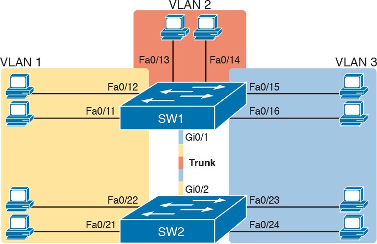
Figure 12: Network with Two Switches and Three VLANs
Example 3 begins by showing the two switches in Figure 12 with the default configuration so that the two switches do not trunk.
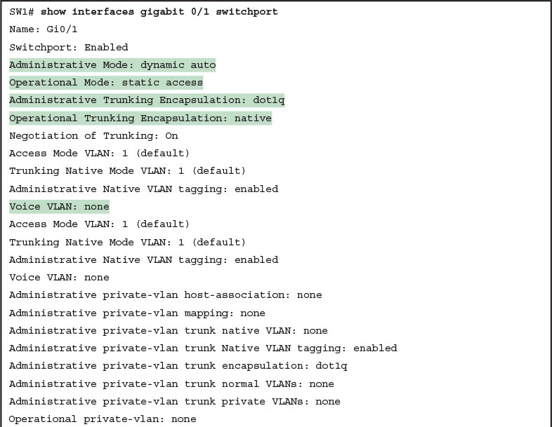
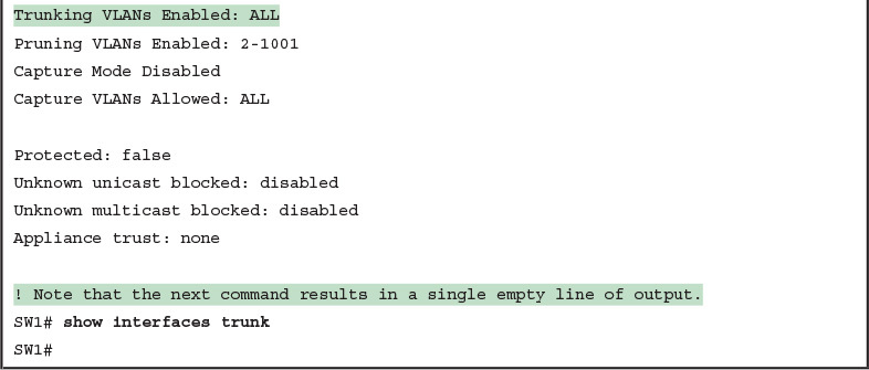
First, focus on the highlighted items from the output of the show interfaces switchport command at the beginning of Example 3. The output lists the default administrative mode setting of dynamic auto. Because SW2 also defaults to dynamic auto, the command lists SW1’s operational status as “access,” meaning that it is not trunking. (“Dynamic auto” tells both switches to sit there and wait on the other switch to start the negotiations.) The third shaded line points out the only supported type of trunking (802.1Q) on this 2960 switch. (On a switch that supports both ISL and 802.1Q, this value would by default list “negotiate,” to mean that the type of encapsulation is negotiated.) Finally, the operational trunking type is listed as “native,” which is a reference to the 802.1Q native VLAN.
The end of the example shows the output of the show interfaces trunk command, but with no output. This command lists information about all interfaces that currently operationally trunk; that is, it lists interfaces that currently use VLAN trunking. With no interfaces listed, this command also confirms that the link between switches is not trunking.
Next, consider Example 4, which shows the new configuration that enables trunking. In this case, SW1 is configured with the switchport mode dynamic desirable command, which asks the switch to both negotiate as well as to begin the negotiation process, rather than waiting on the other device. As soon as the command is issued, log messages appear showing that the interface goes down and then back up again, which happens when the interface transitions from access mode to trunk mode.
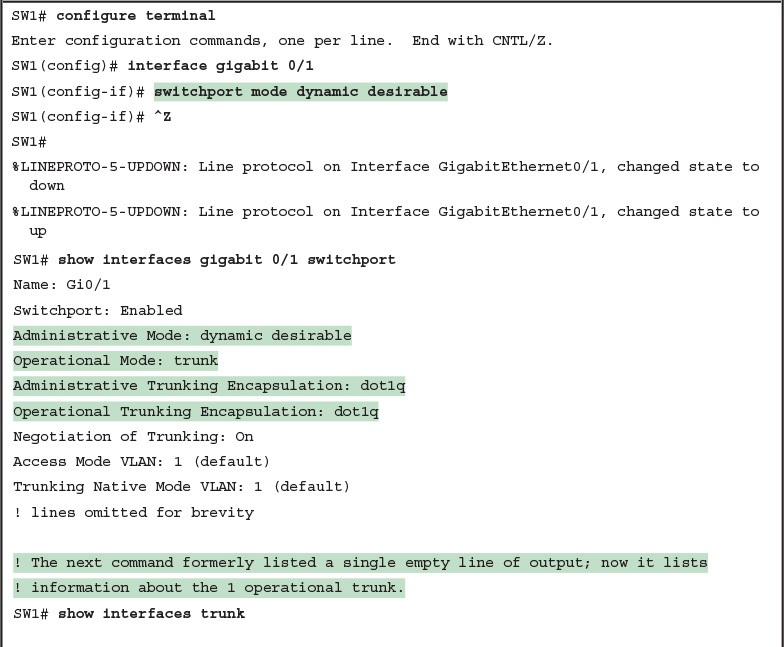
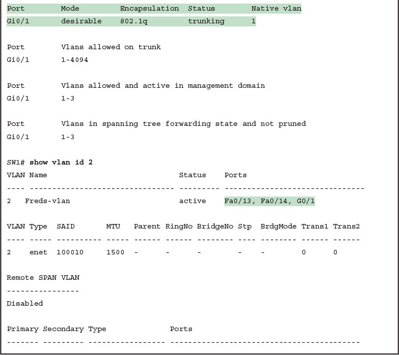
Example 4: SW1 Changes from Dynamic Auto to Dynamic Desirable
To verify whether trunking is working now, the middle of Example 4 lists the show interfaces switchport command. Note that the command still lists the administrative settings, which denote the configured values along with the operational settings, which list what the switch is currently doing. In this case, SW1 now claims to be in an operational mode of trunk, with an operational trunking encapsulation of dot1Q.
The end of the example shows the output of the show interfaces trunk command, which now lists G0/1, confirming that G0/1 is now operationally trunking. The next section discusses the meaning of the output of this command.
For the exams, you should be ready to interpret the output of the show interfaces switchport command, realize the administrative mode implied by the output, and know whether the link should operationally trunk based on those settings. Table 2 lists the combinations of the trunking administrative modes and the expected operational mode (trunk or access) resulting from the configured settings. The table lists the administrative mode used on one end of the link on the left, and the administrative mode on the switch on the other end of the link across the top of the table.
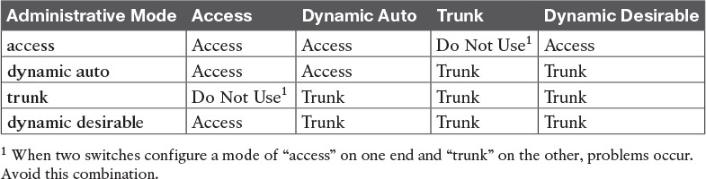
Table 2: Expected Trunking Operational Mode Based on the Configured Administrative Modes
Finally, before leaving the discussion of configuring trunks, Cisco recommends disabling trunk negotiation on most ports for better security. The majority of switch ports on most switches will be used to connect to users. As a matter of habit, you can disable DTP negotiations altogether using the switchport nonegotiate interface subcommand.
Implementing Interfaces Connected to Phones
This next topic is a strange topic, at least in the context of access links and trunk links. In the world of IP telephony, telephones use Ethernet ports to connect to an Ethernet network so they can use IP to send and receive voice traffic sent via IP packets. To make that work, the switch’s Ethernet port acts like an access port—but at the same time, the port acts like a trunk in some ways. This last topic of the lesson works through those main concepts.
Data and Voice VLAN Concepts
Before IP telephony, a PC could sit on the same desk as a phone. The phone happened to use UTP cabling, with that phone connected to some voice device (often called a voice switch or a private branch exchange [PBX]). The PC, of course, connected using a unshielded twisted-pair (UTP) cable to the usual LAN switch that sat in the wiring closet—sometimes in the same wiring closet as the voice switch. Figure 13 shows the idea.
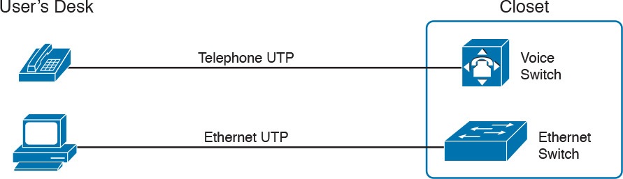
Figure 13: Before IP Telephony: PC and Phone, One Cable Each, Connect to Two Different Devices
The term IP telephony refers to the branch of networking in which the telephones use IP packets to send and receive voice as represented by the bits in the data portion of the IP packet. The phones connect to the network like most other end-user devices, using either Ethernet or Wi-Fi. These new IP phones did not connect via cable directly to a voice switch, instead connecting to the IP network using an Ethernet cable and an Ethernet port built in to the phone. The phones then communicated over the IP network with software that replaced the call setup and other functions of the PBX. (The current products from Cisco that perform this IP telephony control function are called Cisco Unified Communication Manager.)
The migration from using the already-installed telephone cabling, to these new IP phones that needed UTP cables that supported Ethernet, caused some problems in some offices. In particular:
The older non-IP phones used a category of UTP cabling that often did not support 100-Mbps or 1000-Mbps Ethernet.
Most offices had a single UTP cable running from the wiring closet to each desk, but now two devices (the PC and the new IP phone) both needed a cable from the desktop to the wiring closet.
Installing a new cable to every desk would be expensive, plus you would need more switch ports.
To solve this problem, Cisco embedded small three-port switches into each phone.
IP telephones have included a small LAN switch, on the underside of the phone, since the earliest IP telephone products. Figure 14 shows the basic cabling, with the wiring closet cable connecting to one physical port on the embedded switch, the PC connecting with a short patch cable to the other physical port, and the phone’s internal CPU connecting to an internal switch port.
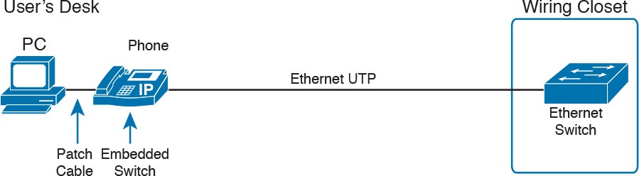
Figure 14: Cabling with an IP Phone, a Single Cable, and an Integrated Switch
Sites that use IP telephony, which includes most every company today, now have two devices off each access port. In addition, Cisco best practices for IP telephony design tell us to put the phones in one VLAN, and the PCs in a different VLAN. To make that happen, the switch port acts a little like an access link (for the PC’s traffic), and a little like a trunk (for the phone’s traffic). The configuration defines two VLANs on that port, as follows:
Data VLAN: Same idea and configuration as the access VLAN on an access port, but defined as the VLAN on that link for forwarding the traffic for the device connected to the phone on the desk (typically the user’s PC).
Voice VLAN: The VLAN defined on the link for forwarding the phone’s traffic. Traffic in this VLAN is typically tagged with an 802.1Q header.
Figure 15 illustrates this design with two VLANs on access ports that support IP telephones.
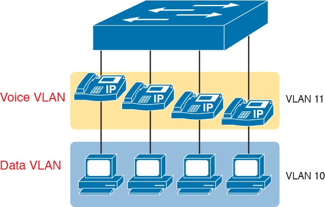
Figure 15: A LAN Design, with Data in VLAN 10 and Phones in VLAN 11
Data and Voice VLAN Configuration and Verification
Configuring a switch port to support IP phones, once you know the planned voice and data VLAN IDs, is easy. Making sense of the show commands once it is configured can be a challenge. The port acts like an access port in many ways. However, with most configuration options, the voice frames flow with an 802.1Q header, so that the link supports frames in both VLANs on the link. But that makes for some different show command output.
Example 5 shows an example. In this case, all four switch ports F0/1–F0/4 begin with default configuration. The configuration adds the new data and voice VLANs. The example then configures all four ports as access ports, and defines the access VLAN, which is also called the data VLAN when discussing IP telephony. Finally, the configuration includes the switchport voice vlan 11 command, which defines the voice VLAN used on the port. The example matches Figure 15, using ports F0/1–F0/4.
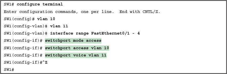
Example 5: Configuring the Voice and Data VLAN on Ports Connected to Phones
NOTE: CDP must be enabled on an interface for a voice access port to work with Cisco IP Phones. CDP is enabled by default, so its configuration is not shown here.
The following list details the configuration steps for easier review and study:
- Step 1. Use the vlan vlan-id command in global configuration mode to create the data and voice VLANs if they do not already exist on the switch.
- Step 2. Configure the data VLAN like an access VLAN, as usual:
- A. Use the interface type number command global configuration mode to move into interface configuration mode.
- B. Use the switchport access vlan id-number command in interface configuration mode to define the data VLAN.
- C. Use the switchport mode access command in interface configuration mode to make this port always operate in access mode (that is, to not trunk).
- Step 3. Use the switchport voice vlan id-number command in interface configuration mode to set the voice VLAN ID.
Verifying the status of a switch port configured like Example 5 shows some different output compared to the pure access port and pure trunk port configurations seen earlier in this lesson. For example, the show interfaces switchport command shows details about the operation of an interface, including many details about access ports. Example 6 shows those details for port F0/4 after the configuration in Example 5 was added.
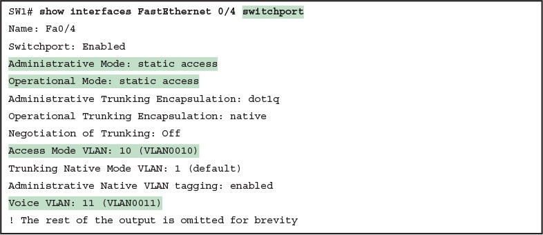
Example 6: Verifying the Data VLAN (Access VLAN) and Voice VLAN
Working through the first three highlighted lines in the output, all those details should look familiar for any access port. The switchport mode access configuration command statically configures the administrative mode to be an access port, so the port of course operates as an access port. Also, as shown in the third highlighted line, the switchport access vlan 10 configuration command defined the access mode VLAN as highlighted here.
The fourth highlighted line shows the one small new piece of information: the voice VLAN ID, as set with the switchport voice vlan 11 command in this case. This small line of output is the only piece of information in the output that differs from the earlier access port examples in this lesson.
These ports act more like access ports than trunk ports. In fact, the show interfaces type number switchport command boldly proclaims, “Operational Mode: static access.” However, one other show command reveals just a little more about the underlying operation with 802.1Q tagging for the voice frames.
As mentioned earlier, the show interfaces trunk command—that is, the command that does not include a specific interface in the middle of the command—lists the operational trunks on a switch. With IP telephony ports, the ports do not show up in the list of trunks either—providing evidence that these links are not treated as trunks. Example 7 shows just such an example.
However, the show interfaces trunk command with the interface listed in the middle of the command, as is also shown in Example 7, does list some additional information. Note that in this case, the show interfaces F0/4 trunk command lists the status as not-trunking, but with VLANs 10 and 11 allowed on the trunk. (Normally, on an access port, only the access VLAN is listed in the “VLANs allowed on the trunk” list in the output of this command.)
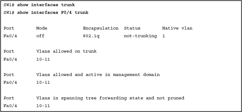
Example 7: Allowed VLAN List and the List of Active VLANs
Summary: IP Telephony Ports on Switches
It might seem like this short topic about IP telephony and switch configuration includes a lot of small twists and turns and trivia, and it does. The most important items to remember are as follows:
- Configure these ports like a normal access port to begin: Configure it as a static access port and assign it an access VLAN.
- Add one more command to define the voice VLAN (switchport voice vlan vlan-id).
- Look for the mention of the voice VLAN ID, but no other new facts, in the output of the show interfaces type number switchport command.
- Look for both the voice and data (access) VLAN IDs in the output of the show interfaces type number trunk command.
- Do not expect to see the port listed in the list of operational trunks as listed by the show interfaces trunk command.

Analyzing Ethernet LAN Designs
INTERNOLD NETWORKS CCNA LIVE WEBCLASS (INCLW)
Analyzing Ethernet LAN Designs
Contents
Analyzing Ethernet LAN Designs
Ethernet defines what happens on each Ethernet link, but the more interesting and more detailed work happens on the devices connected to those links: the network interface cards (NIC) inside devices and the LAN switches.
This lesson takes the Ethernet LAN basics introduced in “Fundamentals of Ethernet LANs,” and dives deeply into many aspects of a modern Ethernet LAN, while focusing on the primary device used to create these LANs: LAN switches.
This lesson breaks down the discussion of Ethernet and LAN switching into two sections.
The first major section looks at the logic used by LAN switches when forwarding Ethernet frames, along with the related terminology.
The second section considers design and implementation issues, as if you were building a new Ethernet LAN in a building or campus.
This second section considers design issues, including using switches for different purposes, when to choose different types of Ethernet links, and how to take advantage of Ethernet autonegotiation.
Analyzing Collision Domains and Broadcast Domains
Ethernet devices, and the logic they use, have a big impact on why engineers design modern LANs in a certain way.
Some of the terms used to describe key design features come from far back in the history of Ethernet, and because of their age, the meaning of each term may or may not be so obvious to someone learning Ethernet today.
This first section of the lesson looks at two of these older terms in particular: collision domain and broadcast domain. And to understand these terms and apply them to modern Ethernet LANs, this section needs to work back through the history of Ethernet a bit, to put some perspective on the meaning behind these terms.
Ethernet Collision Domains
The term collision domain comes from the far back history of Ethernet LANs. To be honest, sometimes people new to Ethernet can get a little confused about what this term really means in the context of a modern Ethernet LAN, in part because modern Ethernet LANs, done properly, can completely prevent collisions.
So to fully understand collision domains, we must first start with a bit of Ethernet history.
This next section of the lesson looks at a few of the historical Ethernet devices, for the purpose of defining a collision domain, and then closing with some comments about how the term applies in a modern Ethernet LAN that uses switches.
10BASE-T with Hub
10BASE-T, introduced in 1990, significantly changed the design of Ethernet LANs, more like the designs seen today. 10BASE-T introduced the cabling model similar to today’s Ethernet LANs, with each device connecting to a centralized device using an unshielded twisted-pair (UTP) cable.
However, 10BASE-T did not originally use LAN switches; instead, the early 10BASE-T networks used a device called an Ethernet hub. (The technology required to build even a basic LAN switch was not yet available at that time.)
Although both a hub and a switch use the same cabling star topology, an Ethernet hub does not forward traffic like a switch. Ethernet hubs use physical layer processing to forward data. A hub does not interpret the incoming electrical signal as an Ethernet frame, look at the source and destination MAC address, and so on.
Basically, a hub acts like a repeater, just with lots of ports. When a repeater receives an incoming electrical signal, it immediately forwards a regenerated signal out all the other ports except the incoming port. Physically, the hub just sends out a cleaner version of the same incoming electrical signal, as shown in Figure 1, with Larry’s signal being repeated out the two ports on the right.

Figure 1: 10BASE-T (with a Hub): The Hub Repeats Out All Other Ports
Because of the physical layer operation used by the hub, the devices attached to the network must use carrier sense multiple access with collision detection (CSMA/CD) to take turns (as introduced at the end of Fundamentals of Ethernet LANs lesson).
Note that the hub itself does not use CSMA/CD logic; the hub always receives an electrical signal and starts repeating a (regenerated) signal out all other ports, with no thought of CSMA/CD.
So, although a hub’s logic works well to make sure all devices get a copy of the original frame, that same logic causes frames to collide.
Figure 2 demonstrates that effect, when the two devices on the right side of the figure send a frame at the same time, and the hub physically transmits both electrical signals out the port to the left (toward Larry).

Figure 2: Hub Operation Causing a Collision
Because a hub makes no attempt to prevent collisions, the devices connected to it all sit within the same collision domain. A collision domain is the set of NICs and device ports for which if they sent a frame at the same time, the frames would collide.
In Figures 1 and Figure 2, all three PCs are in the same collision domain, as well as the hub. Summarizing the key points about hubs:
- The hub acts a multiport repeater, blindly regenerating and repeating any incoming electrical signal out all other ports, even ignoring CSMA/CD rules.
- When two or more devices send at the same time, the hub’s actions cause an electrical collision, making both signals corrupt.
- The connected devices must take turns by using carrier sense multiple access with collision detection (CSMA/CD) logic, so the devices share the bandwidth.
- Hubs create a physical star topology.
Ethernet Transparent Bridges
From a design perspective, the introduction of 10BASE-T was a great improvement over the earlier types of Ethernet. It reduced cabling costs and cable installation costs, and improved the availability percentages of the network.
But sitting here today, thinking of a LAN in which all devices basically have to wait their turn may seem like a performance issue, and it was. If Ethernet could be improved to allow multiple devices to send at the same time without causing a collision, Ethernet performance could be improved.
The first method to allow multiple devices to send at the same time was Ethernet transparent bridges. Ethernet transparent bridges, or simply bridges, made these improvements:
- Bridges sat between hubs and divided the network into multiple collision domains.
- Bridges increase the capacity of the entire Ethernet, because each collision domain is basically a separate instance of CSMA/CD, so each collision domain can have one sender at a time.
Figure 3 shows the effect of building a LAN with two hubs, each separated by a bridge. The resulting two collision domains each support at most 10 Mbps of traffic each, compared to at most 10 Mbps if a single hub were used.

Figure 3: Bridge Creates Two Collision Domains and Two Shared Ethernets
Bridges create multiple collision domains as a side effect of their forwarding logic. A bridge makes forwarding decisions just like a modern LAN switch; in fact, bridges were the predecessors of the modern LAN switch.
Like switches, bridges hold Ethernet frames in memory, waiting to send out the outgoing interface based on CSMA/CD rules. In other cases, the bridge does not even need to forward the frame.
For instance, if Fred sends a frame destined to Barney’s MAC address, then the bridge would never forward frames from the left to the right.
Ethernet Switches and Collision Domains
LAN switches perform the same basic core functions as bridges but at much faster speeds and with many enhanced features. Like bridges, switches segment a LAN into separate collision domains, each with its own capacity.
And if the network does not have a hub, each single link in a modern LAN is considered its own collision domain, even if no collisions can actually occur in that case.
For example, Figure 4 shows a simple LAN with a switch and four PCs. The switch creates four collision domains, with the ability to send at 100 Mbps in this case on each of the four links. And with no hubs, each link can run at full duplex, doubling the capacity of each link.

Figure 4: Switch Creates Four Collision Domains and Four Ethernet Segments
Now take a step back for a moment and think about some facts about modern Ethernet LANs. Today, you build Ethernet LANs with Ethernet switches, not with Ethernet hubs or bridges. The switches connect to each other. And every single link is a separate collision domain.
As strange as it sounds, each of those collision domains in a modern LAN may also never have a collision. Any link that uses full duplex—that is, both devices on the link use full duplex—does not have collisions.
In fact, running with full duplex is basically this idea: No collisions can occur between a switch and a single device, so we can turn off CSMA/CD by running full duplex.
NOTE: The routers in a network design also create separate collision domains, because frames entering or exiting one router LAN interface do not collide with frames on another of the router’s LAN interfaces.
The Impact of Collisions on LAN Design
So, what is the useful takeaway from this discussion about collision domains? A long time ago, collisions were normal in Ethernet, so analyzing an Ethernet design to determine where the collision domains were was useful.
On the other end of the spectrum, a modern campus LAN that uses only switches (and no hubs or transparent bridges), and full duplex on all links, has no collisions at all. So does the collision domain term still matter today? And do we need to think about collisions even still today?
In a word, the term collision domain still matters, and collisions still matter, in that network engineers need to be ready to understand and troubleshoot exceptions.
Whenever a port that could use full duplex (therefore avoiding collisions) happens to use half duplex—by incorrect configuration, by the result of autonegotiation, or any other reason—collisions can now occur. In those cases, engineers need to be able identify the collision domain.
Summarizing the key points about collision domains:
- LAN switches place each separate interface into a separate collision domain.
- LAN bridges, which use the same logic as switches, placed each interface into a separate collision domain.
- Routers place each LAN interface into a separate collision domain. (The term collision domain does not apply to WAN interfaces.)
- LAN hubs do not place each interface into a separate collision domain.
- A modern LAN, with all LAN switches and routers, with full duplex on each link, would not have collisions at all.
- In a modern LAN with all switches and routers, even though full duplex removes collisions, think of each Ethernet link as a separate collision domain when the need to troubleshoot arises.
Figure 5 shows an example with a design that includes hubs, bridges, switches, and routers—a design that you would not use today, but it makes a good backdrop to remind us about which devices create separate collision domains.

Figure 5: Example of a Hub Not Creating Multiple Collision Domains, While Others Do
Ethernet Broadcast Domains
Take any Ethernet LAN, and pick any device. Then think of that device sending an Ethernet broadcast. An Ethernet broadcast domain is the set of devices to which that broadcast is delivered.
To begin, think about a modern LAN for a moment, and where a broadcast frame flows. Imagine that all the switches still used the switch default to put each interface into VLAN 1.
As a result, a broadcast sent by any one device would be flooded to all devices connected to all switches (except for the device that sent the original frame).
For instance, in Figure 6, under the assumption that all ports are still assigned to VLAN 1, a broadcast would flow to all the devices shown in the figure.

Figure 6: A Single Large Broadcast Domain
Of all the common networking devices discussed in this lesson, only a router does not forward a LAN broadcast. Hubs of course forward broadcasts, because hubs do not even think about the electrical signal as an Ethernet frame. Bridges and switches use the same forwarding logic, flooding LAN broadcasts.
Routers, as a side effect of their routing logic, do not forward Ethernet broadcast frames, so they separate a network into separate broadcast domains.
Figure 7 collects those thoughts into a single example.

Figure 7: Broadcast Domains Separated by a Router
By definition, broadcasts sent by a device in one broadcast domain are not forwarded to devices in another broadcast domain. In this example, there are two broadcast domains. The router does not forward a LAN broadcast sent by a PC on the left to the network segment on the right.
Virtual LANs
Routers create multiple broadcast domains mostly as a side effect of how IP routing works. While a network designer might set about to use more router interfaces for the purpose of making a larger number of smaller broadcast domains, that plan quickly consumes router interfaces. But a better tool exists, one that is integrated into LAN switches and consumes no additional ports: virtual LANs (VLAN).
By far, VLANs give the network designer the best tool for designing the right number of broadcast domains, of the right size, with the right devices in each. To appreciate how VLANs do that, you must first think about one specific definition of what a LAN is:
A LAN consists of all devices in the same broadcast domain.
With VLANs, a switch configuration places each port into a specific VLAN. The switches create multiple broadcast domains by putting some interfaces into one VLAN and other interfaces into other VLANs.
The switch forwarding logic does not forward frames from a port in one VLAN out a port into another VLAN—so the switch separates the LAN into separate broadcast domains. Instead, routers must forward packets between the VLANs by using routing logic. So, instead of all ports on a switch forming a single broadcast domain, the switch separates them into many, based on configuration.
For perspective, think about how you would create two different broadcast domains with switches if the switches had no concept of VLANs. Without any knowledge of VLANs, a switch would receive a frame on one port and flood it out all the rest of its ports. Therefore, to make two broadcast domains, two switches would be used—one for each broadcast domain, as shown in Figure 8.

Figure 8: Sample Network with Two Broadcast Domains and No VLANs
Alternatively, with a switch that understands VLANs, you can create multiple broadcast domains using a single switch. All you do is put some ports in one VLAN and some in the other. (The Cisco Catalyst switch interface subcommand to do so is switchport access vlan 2, for instance, to place a port into VLAN 2.)
Figure 9 shows the same two broadcast domains as in Figure 8, now implemented as two different VLANs on a single switch.

Figure 9: Sample Network with Two VLANs Using One Switch
This section briefly introduces the concept of VLANs, but the lesson, “Implementing Ethernet Virtual LANs,” discusses VLANs in more depth, including the details of how to configure VLANs in campus LANs.
The Impact of Broadcast Domains on LAN Design
Modern LAN designs try to avoid collisions, because collisions make performance worse. There is no benefit to keeping collisions in the network. However, a LAN design cannot remove broadcasts, because broadcast frames play an important role in many protocols.
So when thinking about broadcast domains, the choices are more about tradeoffs rather than designing to remove broadcasts.
For just one perspective, just think about the size of a broadcast domain—that is, the number of devices in the same broadcast domain. A small number of large broadcast domains can lead to poor performance for the devices in that broadcast domain. However, moving in the opposite direction, to making a large number of broadcast domains each with just a few devices, leads to other problems.
Consider the idea of a too-large broadcast domain for a moment. When a host receives a broadcast, the host must process the received frame. All hosts need to send some broadcasts to function properly, so when a broadcast arrives, the NIC must interrupt the computer’s CPU to give the incoming message to the CPU. The CPU must spend time thinking about the received broadcast frame. (For example, IP Address Resolution Protocol [ARP] messages are LAN broadcasts, as mentioned in the lesson “Fundamentals of IPv4 Addressing and Routing.”)
So, broadcasts happen, which is good, but broadcasts do require all the hosts to spend time processing each broadcast frame. The more devices in the same broadcast domain, the more unnecessary interruptions of each device’s CPU.
This section does not try to give a sweeping review of all VLAN design tradeoffs. Instead, you can see that the size of a VLAN should be considered, but many other factors come in to play as well. How big are the VLANs? How are the devices grouped? Do VLANs span across all switches or just a few? Is there any apparent consistency to the VLAN design, or is it somewhat haphazard? Answering these questions helps reveal what the designer was thinking, as well as what the realities of operating a network may have required.
Summarizing the main points about broadcast domains:
- Broadcasts exists, so be ready to analyze a design to define each broadcast domain, that is, each set of devices whose broadcasts reach the other devices in that domain.
- VLANs by definition are broadcast domains created though configuration.
- Routers, because they do not forward LAN broadcasts, create separate broadcast domains off their separate Ethernet interfaces.
Analyzing Campus LAN Topologies
The term campus LAN refers to the LAN created to support the devices in a building or in multiple buildings in somewhat close proximity to one another. For example, a company might lease office space in several buildings in the same office park.
The network engineers can then build a campus LAN that includes switches in each building, plus Ethernet links between the switches in the buildings, to create a larger campus LAN.
When planning and designing a campus LAN, the engineers must consider the types of Ethernet available and the cabling lengths supported by each type. The engineers also need to choose the speeds required for each Ethernet segment.
In addition, some thought needs to be given to the idea that some switches should be used to connect directly to end-user devices, whereas other switches might need to simply connect to a large number of these end-user switches.
Finally, most projects require that the engineer consider the type of equipment that is already installed and whether an increase in speed on some segments is worth the cost of buying new equipment.
This second of three major sections discusses the topology of a campus LAN design.
Network designers do not just plug in devices to any port and connect switches to each other in an arbitrary way, like you might do with a few devices on the same table in a lab.
Instead, there are known better ways to design the topology of a campus LAN, and this section introduces some of the key points and terms.
The last major section of the lesson then looks at how to choose which Ethernet standard to use for each link in that campus LAN design, and why you might choose one versus another.
Two-Tier Campus Design (Collapsed Core)
To sift through all the requirements for a campus LAN, and then have a reasonable conversation about it with peers, most Cisco-oriented LAN designs use some common terminology to refer to the design. For this lesson’s purposes, you should be aware of some of the key campus LAN design terminology.
The Two-Tier Campus Design
Figure 10 shows a typical design of a large campus LAN, with the terminology included in the figure. This LAN has around 1000 PCs connected to switches that support around 25 ports each. Explanations of the terminology follow the figure.

Campus LAN with Design Terminology Listed
Cisco uses three terms to describe the role of each switch in a campus design: access, distribution, and core. The roles differ based on whether the switch forwards traffic from user devices and the rest of the LAN (access), or whether the switch forwards traffic between other LAN switches (distribution and core).
Access switches connect directly to end users, providing user device access to the LAN. Access switches normally send traffic to and from the end-user devices to which they are connected and sit at the edge of the LAN.
Distribution switches provide a path through which the access switches can forward traffic to each other. By design, each of the access switches connects to at least one distribution switch, typically to two distribution switches for redundancy.
The distribution switches provide the service of forwarding traffic to other parts of the LAN. Note that most designs use at least two uplinks to two different distribution switches (as shown in Figure 10) for redundancy.
The figure shows a two-tier design, with the tiers being the access tier (or layer) and the distribution tier (or layer). A two-tier design solves two major design needs:
- Provides a place to connect end-user devices (the access layer, with access switches)
- Connects the switches with a reasonable number of cables and switch ports by connecting all 40 access switches to two distribution switches
Topology Terminology Seen Within a Two-Tier Design
The exam topics happen to list a couple of terms about LAN and WAN topology and design, so this is a good place to pause to discuss those terms for a moment.
First, consider these more formal definitions of four topology terms:
- Star: A design in which one central device connects to several others, so that if you drew the links out in all directions, the design would look like a star with light shining in all directions.
- Full mesh: For any set of network nodes, a design that connects a link between each pair of nodes.
- Partial mesh: For any set of network nodes, a design that connects a link between some pairs of nodes, but not all. In other words, a mesh that is not a full mesh.
- Hybrid: A design that combines topology design concepts into a larger (typically more complex) design.
Armed with those formal definitions, note that the two-tier design is indeed a hybrid design that uses both a star topology at the access layer and a partial mesh at the distribution layer. To see why, consider Figure 11.
It redraws a typical access layer switch, but instead of putting the PCs all below the switch, it spreads them around the switch. Then on the right, a similar version of the same drawing shows why the term star might be used—the topology looks a little like a child’s drawing of a star.

Figure 11: The Star Topology Design Concept in Networking
The distribution layer creates a partial mesh. If you view the access and distribution switches as nodes in a design, some nodes have a link between them, and some do not. Just refer to Figure 10 and note that, by design, none of the access layer switches connect to each other.
Finally, a design could use a full mesh. However, for a variety of reasons beyond the scope of the design discussion here, a campus design typically does not need to use the number of links and ports required by a full mesh design. However, just to make the point, first consider how many links and switch ports would be required for a single link between nodes in a full mesh, with six nodes, as shown in Figure 12.

Figure 12: Using a Full Mesh at the Distribution Layer, 6 Switches, 15 Links
Even with only six switches, a full mesh would consume 15 links (and 30 switch ports—two per link).
Now think about a full mesh at the distribution layer for a design like Figure 10, with 40 access switches and two distribution switches. Rather than drawing it and counting it, the number of links is calculated with this old math formula from high school: N(N – 1) / 2, or in this case, 42 * 41 / 2 = 861 links, and 1722 switch ports consumed among all switches.
For comparison’s sake, the partial mesh design of Figure 10, with a pair of links from each access switch to each distribution switch, requires only 160 links and a total of 320 ports among all switches.
Three-Tier Campus Design (Core)
The two-tier design of Figure 10, with a partial mesh of links at the distribution layer, happens to be the most common campus LAN design. It also goes by two common names: a two-tier design (for obvious reasons), and a collapsed core (for less obvious reasons).
The term collapsed core refers to the fact that the two-tier design does not have a third tier, the core tier. This next topic examines a three-tier design that does have a core, for perspective.
Imagine your campus has just two or three buildings. Each building has a two-tier design inside the building, with a pair of distribution switches in each building and access switches spread around the building as needed. How would you connect the LANs in each building?
Well, with just a few buildings, it makes sense to simply cable the distribution switches together, as shown in Figure 13.

Figure 13: Two-Tier Building Design, No Core, Three Buildings
The design in Figure 13 works well, and many companies use this design. Sometimes the center of the network uses a full mesh, sometimes a partial mesh, depending on the availability of cables between the buildings.
However, a design with a third tier (a core tier) saves on switch ports and on cables in larger designs. And note that with the links between buildings, the cables run outside, are often more expensive to install, are almost always fiber cabling with more expensive switch ports, so conserving the number of cables used between buildings can help reduce costs.
A three-tier core design, unsurprisingly at this point, adds a few more switches (core switches), which provide one function: to connect the distribution switches. Figure 14 shows the migration of the Figure 13 collapsed core (that is, a design without a core) to a three-tier core design.

Figure 13: Three-Tier Building Design (Core Design), Three Buildings
NOTE:The core switches sit in the middle of the figure. In the physical world, they often sit in the same room as one of the distribution switches, rather than in some purpose-built room in the middle of the office park. The figure focuses more on the topology rather than the physical location.
By using a core design, with a partial mesh of links in the core, you still provide connectivity to all parts of the LAN, and to the routers that send packets over the WAN, just with fewer links between buildings.
The following list summarizes the terms that describe the roles of campus switches:
- Access: Provides a connection point (access) for end-user devices. Does not forward frames between two other access switches under normal circumstances.
- Distribution: Provides an aggregation point for access switches, providing connectivity to the rest of the devices in the LAN, forwarding frames between switches, but not connecting directly to end-user devices.
- Core: Aggregates distribution switches in very large campus LANs, providing very high forwarding rates for the larger volume of traffic due to the size of the network.
Topology Design Terminology
The CCNA exam topics specifically mention several network design terms related to topology. This next topic summarizes those key terms to connect the terms to the matching ideas.
First, consider Figure 15, which shows a few of the terms. First, on the left, drawings often show access switches with a series of cables, parallel to each other. However, an access switch and its access links is often called a star topology.
Why? Look at the redrawn access switch in the center of the figure, with the cables radiating out from the center. It does not look like a real star, but it looks a little like a child’s drawing of a star, hence the term star topology.

Figure 15: LAN Design Terminology
The right side of the figure repeats a typical two-tier design, focusing on the mesh of links between the access and distribution switches. Any group of nodes that connect with more links than a star topology is typically called a mesh.
In this case, the mesh is a partial mesh, because not all nodes have a direct link between each other.
A design that connects all nodes with a link would be a full mesh.
Real networks make use of these topology ideas, but often a network combines the ideas together.
For instance, the right side of Figure 14 combines the star topology of the access layer with the partial mesh of the distribution layer. So you might hear these designs that combine concepts called a hybrid design.
Analyzing LAN Physical Standard Choices
When you look at the design of a network designed by someone else, you can look at all the different types of cabling used, the different types of switch ports, and the Ethernet standards used in each case. Then ask yourself: Why did they choose a particular type of Ethernet link for each link in the network? Asking that question, and investigating the answer, starts to reveal much about building the physical campus LAN.
The IEEE has done an amazing job developing Ethernet standards that give network designers many options. Two themes in particular have helped Ethernet grow over the long term:
- The IEEE has developed many additional 802.3 standards for different types of cabling, different cable lengths, and for faster speeds.
- All the physical standards rely on the same consistent data-link details, with the same standard frame formats. That means that one Ethernet LAN can use many types of physical links to meet distance, budget, and cabling needs.
For example, think about the access layer of the generic design drawings, but now think about cabling and Ethernet standards. In practice, access layer switches sit in a locked wiring closet somewhere on the same floor as the end user devices.
Electricians have installed unshielded twisted-pair (UTP) cabling used at the access layer, running from that wiring closet to each wall plate at each office, cubicle, or any place where an Ethernet device might need to connect to the LAN. The type and quality of the cabling installed between the wiring closet and each Ethernet outlet dictate what Ethernet standards can be supported.
Certainly, whoever designed the LAN at the time the cabling was installed thought about what type of cabling was needed to support the types of Ethernet physical standards that were going to be used in that LAN.
Ethernet Standards
Over time, the IEEE has continued to develop and release new Ethernet standards, for new faster speeds and to support new and different cabling types and cable lengths. Figure 16 shows some insight into Ethernet speed improvements over the years.
The early standards up through the early 1990s ran at 10 Mbps, with steadily improving cabling and topologies. Then, with the introduction of Fast Ethernet (100 Mbps) in 1995, the IEEE began ramping up the speeds steadily over the next few decades, continuing even until today.

Figure 16: Ethernet Standards Timeline
NOTE: Often, the IEEE first introduces support for the next higher speed using some forms of fiber optic cabling, and later, sometimes many years later, the IEEE completes the work to develop standards to support the same speed on UTP cabling. Figure 16 shows the earliest standards for each speed, no matter what cabling.
When the IEEE introduces support for a new type of cabling, or a faster speed, they create a new standard as part of 802.3. These new standards have a few letters behind the name. So, when speaking of the standards, sometimes you might refer to the standard name (with letters).
For instance, the IEEE standardized Gigabit Ethernet support using inexpensive UTP cabling in standard 802.3ab. However, more often, engineers refer to that same standard as 1000BASE-T or simply Gigabit Ethernet. Table 1 lists some of the IEEE 802.3 physical layer standards and related names for perspective.

Table 1: IEEE Physical Layer Standards
Choosing the Right Ethernet Standard for Each Link
When designing an Ethernet LAN, you can and should think about the topology, with an access layer, a distribution layer, and possibly a core layer. But thinking about the topology does not tell you which specific standards to follow for each link. Ultimately, you need to pick which Ethernet standard to use for each link, based on the following kinds of facts about each physical standard:
- The speed
- The maximum distance allowed between devices when using that standard/cabling
- The cost of the cabling and switch hardware
- The availability of that type of cabling already installed at your facilities
Consider the three most common types of Ethernet today (10BASE-T, 100BASE-T, and 1000BASE-T). They all have the same 100-meter UTP cable length restriction. They all use UTP cabling.
However, not all UTP cabling meets the same quality standard, and as it turns out, the faster the Ethernet standard, the higher the required cable quality category needed to support that standard. As a result, some buildings might have better cabling that supports speeds up through Gigabit Ethernet, whereas some buildings may support only Fast Ethernet.
The Telecommunications Industry Association (TIA; tiaonline.org) defines Ethernet cabling quality standards. Each Ethernet UTP standard lists a TIA cabling quality (called a category) as the minimum category that the standard supports.
For example, 10BASE-T allows for Category 3 (CAT3) cabling or better. 100BASE-T requires higher-quality CAT5 cabling, and 1000BASE-T requires even higher-quality CAT5e cabling. (The TIA standards follow a general “higher number is better cabling” in their numbering.)
For instance, if an older facility had only CAT5 cabling installed between the wiring closets and each cubicle, the engineers would have to consider upgrading the cabling to fully support Gigabit Ethernet. Table 2 lists the more common types of Ethernet and their cable types and length limitations.

Ethernet Types, Media, and Segment Lengths (Per IEEE)
Ethernet defines standards for using fiber optic cables as well. Fiber optic cables include ultrathin strands of glass through which light can pass. To send bits, the switches can alternate between sending brighter and dimmer light to encode 0s and 1s on the cable.
Generally comparing optical cabling versus UTP cabling Ethernet standards, two obvious points stand out. Optical standards allow much longer cabling, while generally costing more for the cable and the switch hardware components. Optical cables experience much less interference from outside sources compared to copper cables, which allows for longer distances.
When considering optical Ethernet links, many standards exist, but with two general categories. Comparing the two, the cheaper options generally support distances into the hundreds of meters, using less expensive light-emitting diodes (LED) to transmit data. Other optical standards support much longer distances into multiple kilometers, using more expensive cabling and using lasers to transmit the data. The trade-off is basic: For a given link, how long does the cable need to run, what standards support that distance, and which is the least expensive to meet that need?
In reality, most engineers remember only the general facts from tables like Table 2: 100 meters for UTP, about 500 meters for multimode fiber, and about 5000 meters for some single mode fiber Ethernet standards. When it is time to get serious about designing the details of each link, the engineer must get into the details, calculating the length of each cable based on its path through the building, and so on.
Wireless LANs Combined with Wired Ethernet
Modern campus LANs include a large variety of wireless devices that connect to the access layer of the LAN. As it turns out, Cisco organizes wireless LANs into a separate certification track—CCNA, CCNP, and CCIE Wireless—so the CCNA R&S track has traditionally had only a little wireless LAN coverage. The current version of the exams are no different, with this one exam CCNA R&S topic mentioning wireless LANs:
Describe the impact of infrastructure components in an enterprise network: Access points and wireless controllers
Do not let that small mention of wireless technology make you think that wireless is less important than Ethernet. In fact, there may be more wireless devices than wired at the access layer of today’s enterprise networks. Both are important; Cisco just happens to keep the educational material for wireless in a separate certification track.
This last topic in the lesson examines that one exam topic that mentions two wireless terms.
Home Office Wireless LANs
First, the IEEE defines both Ethernet LANs and Wireless LANs. In case it was not obvious yet, all Ethernet standards use cables—that is, Ethernet defines wired LANs. The IEEE 802.11 working group defines Wireless LANs, also called Wi-Fi per a trademarked term from the Wi-Fi Alliance (wi-fi.org), a consortium that helps to encourage wireless LAN development in the marketplace.
Most of you have used Wi-Fi, and may use it daily. Some of you may have set it up at home, with a basic setup as shown in Figure 17. In a home, you probably used a single consumer device called a wireless router. One side of the device connects to the Internet, while the other side connects to the devices in the home. In the home, the devices can connect either with Wi-Fi or with a wired Ethernet cable.

Figure 17: A Typical Home Wired and Wireless LAN
While the figure shows the hardware as a single router icon, internally, that one wireless router acts like three separate devices you would find in an enterprise campus:
- An Ethernet switch, for the wired Ethernet connections
- A wireless access point (AP), to communicate with the wireless devices and forward the frames to/from the wired network
- A router, to route IP packets to/from the LAN and WAN (Internet) interfaces
Figure 18 repeats the previous figure, breaking out the internal components as if they were separate physical devices, just to make the point that a single consumer wireless router acts like several different devices.

Figure 18: A Representation of the Functions Inside a Consumer Wireless Routing Product
In a small office/home office (SOHO) wireless LAN, the wireless AP acts autonomously, doing all the work required to create and control the wireless LAN (WLAN). (In most enterprise WLANs, the AP does not act autonomously.) In other words, the autonomous AP communicates with the various wireless devices using 802.11 protocols and radio waves.
It uses Ethernet protocols on the wired side. It converts between the differences in header formats between 802.11 and 802.3 frames before forwarding to/from 802.3 Ethernet and 802.11 wireless frames.
Beyond those basic forwarding actions, the autonomous AP must perform a variety of control and management functions. The AP authenticates new devices, defines the name of the WLAN (called a service set ID, or SSID), and other details.
Enterprise Wireless LANs and Wireless LAN Controllers
If you connect to your WLAN at home from your tablet, phone, or laptop, and then walk down the street with that same device, you expect to lose your Wi-Fi connection at some point. You do not expect to somehow automatically connect to a neighbor’s Wi-Fi network, particularly if they did the right thing and set up security functions on their AP to prevent others from accessing their home Wi-Fi network. The neighborhood does not create one WLAN supported by the devices in all the houses and apartments; instead, it has lots of little autonomous WLANs.
However, in an enterprise, the opposite needs to happen. We want people to be able to roam around the building and office campus and keep connected to the Wi-Fi network. This requires many APs, which work together rather than autonomously to create one wireless LAN.
First, think about the number of APs an enterprise might need. Each AP can cover only a certain amount of space, depending on a large number of conditions and the wireless standard. (The size varies, but the distances sit in the 100 to 200 feet range.) At the same time, you might have the opposite problem; you may just need lots of APs in a small space, just to add capacity to the WLAN. Much of the time spent designing WLANs revolves around deciding how many APs to place in each space, and of what types, to handle the traffic.
NOTE: If you have not paid attention before, start looking around the ceilings of any new buildings you enter, even retail stores, and look for their wireless APs.
Each AP must then connect to the wired LAN, because most of the destinations that wireless users need to communicate with sit in the wired part of the network. In fact, the APs typically sit close to where users sit, for obvious reasons, so the APs connect to the same access switches as the end users, as shown in Figure 19.

Figure 19: Campus LAN, Multiple Lightweight APs, with Roaming
Now imagine that is you at the bottom of the figure. Your smartphone has Wi-Fi enabled, so that when you walk into work, your phone automatically connects to the company WLAN. You roam around all day, going to meetings, lunch, and so on. All day long you stay connected to the company WLAN, but your phone connects to and uses many different APs.
Supporting roaming and other enterprise WLAN features by using autonomous APs can be difficult at best. You could imagine that if you had a dozen APs per floor, you might have hundreds of APs in a campus—all of which need to know about that one WLAN.
The solution: remove all the control and management features from the APs, and put them in one centralized place, called a Wireless Controller, or Wireless LAN Controller (WLC). The APs no longer act autonomously, but instead act as lightweight APs (LWAPs), just forwarding data between the wireless LAN and the WLC. All the logic to deal with roaming, defining WLANs (SSIDs), authentication, and so on happens in the centralized WLC rather than on each AP. Summarizing:
- Wireless LAN controller: Controls and manages all AP functions (for example, roaming, defining WLANs, authentication)
- Lightweight AP (LWAP): Forwards data between the wired and wireless LAN, and specifically forwarding data through the WLC using a protocol like Control And Provisioning of Wireless Access Points (CAPWAP)
With the WLC and LWAP design, the combined LWAPs and WLC can create one big wireless network, rather than creating a multitude of disjointed wireless networks. The key to making it all work is that all wireless traffic flows through the WLC, as shown in Figure 20. (The LWAPs commonly use a protocol called CAPWAP, by the way.)

Figure 20: Campus LAN, Multiple Lightweight APs, with Roaming
By forwarding all the traffic through the WLC, the WLC can make the right decisions across the enterprise. For example, you might create a marketing WLAN, an engineering WLAN, and so on, and all the APs know about and support those multiple different WLANs.
Users that connect to the engineering WLAN should use the same authentication rules regardless of which AP they use—and the WLC makes that possible. Or consider roaming for a moment. If at one instant a packet arrives for your phone, and you are associated with AP1, and when the next packet arrives over the wired network you are now connected to AP4, how could that packet be delivered through the network?
Well, it always goes to the WLC, and because the WLC keeps in contact with the APs and knows that your phone just roamed to another AP, the WLC knows where to forward the packet.

Configuring Switch Interfaces
INTERNOLD NETWORKS CCNA LIVE WEBCLASS (INCLW)
Configuring Switch Interfaces
Contents
Configuring Switch Interfaces
So far, you have learned the skills to navigate the command-line interface (CLI) and use commands that configure and verify switch features.
You learned about the primary purpose of a switch—forwarding Ethernet frames—and learned how to see that process in action by looking at the switch MAC address table.
After learning about the switch data plane in the lesson, “Analyzing Ethernet LAN Switching,” you learned a few management plane features in the lesson, “Configuring Basic Switch Management,” like how to configure the switch to support Telnet and Secure Shell (SSH) by configuring IP address and login security.
In this lesson, you pick up tools that loosely fit in the switch control plane.
First, this lesson shows how you can configure and change the operation of switch interfaces: how to change the speed, duplex, or even disable the interface.
The second half then shows how to add a security feature called port security, which monitors the source MAC address of incoming frames, deciding which frames are allowed and which cause a security violation.
Configuring Switch Interfaces
IOS uses the term interface to refer to physical ports used to forward data to and from other devices. Each interface can be configured with several settings, each of which might differ from interface to interface. IOS uses interface subcommands to configure these settings.
Each of these settings may be different from one interface to the next, so you would first identify the specific interface, and then configure the specific setting.
This section begins with a discussion of three relatively basic per-interface settings: the port speed, duplex, and a text description. Following that, the text takes a short look at a pair of the most common interface subcommands: the shutdown and no shutdown commands, which administratively disable and enable the interface, respectively.
This section ends with a discussion about autonegotiation concepts, which in turn dictates what settings a switch chooses to use when using autonegotiation.
Configuring Speed, Duplex, and Description
Switch interfaces that support multiple speeds (10/100 and 10/100/1000 interfaces), by default, will autonegotiate what speed to use. However, you can configure the speed and duplex settings with the duplex {auto | full | half} and speed {auto | 10 | 100 | 1000} interface subcommands. Simple enough.
Most of the time, using autonegotiation makes good sense, so when you set the duplex and speed, you typically have a good reason to do so. For instance, maybe you want to set the speed to the fastest possible on links between switches just to avoid the chance that auto-negotiation chooses a slower speed.
The description text interface subcommand lets you add a text description to the interface. For instance, if you have good reason to configure the speed and duplex on a port, maybe add a description that says why you did. Example 1 shows how to configure duplex and speed, as well as the description command, which is simply a text description that can be configured by the administrator.
Image

Example 1: Configuring speed, duplex, and description on Switch Emma
First, focus on the mechanics of moving around in configuration mode again by looking closely at the command prompts. The various interface commands move the user from global mode into interface configuration mode for a specific interface. For instance, the example configures the duplex, speed, and description commands all just after the interface FastEthernet 0/1 command, which means that all three of those configuration settings apply to interface Fa0/1, and not to the other interfaces.
The show interfaces status command lists much of the detail configured in Example 1, even with only one line of output per interface. Example 2 shows an example, just after the configuration in Example 1 was added to the switch.


Example 2: Displaying Interface Status
Working through the output in the example:
FastEthernet 0/1 (Fa0/1): This output lists the first few characters of the configured description. It also lists the configured speed of 100 and duplex full per the speed and duplex commands in Example 1. However, it also states that Fa0/1 has a status of notconnect, meaning that the interface is not currently working. (That switch port did not have a cable connected when collecting this example, on purpose.)
FastEthernet 0/2 (Fa0/2): Example 1 did not configure this port at all. This port had all default configuration. Note that the “auto” text under the speed and duplex heading means that this port will attempt to autonegotiate both settings when the port comes up. However, this port also does not have a cable connected (again on purpose, for comparison).
FastEthernet 0/4 (Fa0/4): Like Fa0/2, this port has all default configuration, but was cabled to another working device to give yet another contrasting example. This device completed the autonegotiation process, so instead of “auto” under the speed and duplex headings, the output lists the negotiated speed and duplex (a-full and a-100). Note that the text includes the a- to mean that the listed speed and duplex values were autonegotiated.
Configuring Multiple Interfaces with the interface range Command
The bottom of the configuration in Example 1 shows a way to shorten your configuration work when making the same setting on multiple consecutive interfaces. To do so, use the interface range command. In the example, the interface range FastEthernet 0/11 - 20 command tells IOS that the next subcommand(s) apply to interfaces Fa0/11 through Fa0/20. You can define a range as long as all interfaces are the same type and are numbered consecutively.
NOTE: This lesson spells out all parameters fully to avoid confusion. However, most everyone abbreviates what they type in the CLI to the shortest unique abbreviation. For instance, the configuration commands int f0/1 and int ran f0/11 - 20 would also be acceptable.
IOS does not actually put the interface range command into the configuration. Instead, it acts as if you had typed the subcommand under every single interface in the specified range.
Example 3 shows an excerpt from the show running-config command, listing the configuration of interfaces F0/11–12 from the configuration in Example 1.
The example shows the same description command on both interfaces; to save space the example did not bother to show all 10 interfaces that have the same description text.

Example 3: How IOS Expands the Subcommands Typed After interface range
Administratively Controlling Interface State with shutdown
As you might imagine, network engineers need a way to bring down an interface without having to travel to the switch and remove a cable. In short, we need to be able to decide which ports should be enabled, and which should be disabled.
In an odd turn of phrase, Cisco uses two interface subcommands to configure the idea of administratively enabling and disabling an interface: the shutdown command (to disable), and the no shutdown command (to enable). While the no shutdown command might seem like an odd command to enable an interface at first, you will use this command a lot in lab, and it will become second nature. (Most people in fact use the abbreviations shut and no shut.)
Example 4 shows an example of disabling an interface using the shutdown interface subcommand. In this case, switch SW1 has a working interface F0/1. The user connects at the console and disables the interface. IOS generates a log message each time an interface fails or recovers, and log messages appear at the console, as shown in the example.

Example 4: Administratively Disabling an Interface with shutdown
To bring the interface back up again, all you have to do is follow the same process but use the no shutdown command instead.
Before leaving the simple but oddly named shutdown/no shutdown commands, take a look at two important show commands that list the status of a shutdown interface. The show interfaces status command lists one line of output per interface, and when shut down, lists the interface status as “disabled.” That makes logical sense to most people. The show interfaces command (without the status keyword) lists many lines of output per interface, giving a much more detailed picture of interface status and statistics. With that command, the interface status comes in two parts, with one part using the phrase “administratively down,” matching the highlighted log message in Example 4.
Example 5 shows an example of each of these commands. Note that both examples also use the F0/1 parameter (short for Fast Ethernet0/1), which limits the output to the messages about F0/1 only. Also note that F0/1 is still shut down at this point.


Example 5: The Different Status Information About Shutdown in Two Different show Commands
Removing Configuration with the no Command
In some cases, the commands are not the end goal, and the text is attempting to teach you something about how the CLI works. This next short topic is more about the process than about the commands.
With some IOS configuration commands (but not all), you can revert to the default setting by issuing a no version of the command. What does that mean? Let me give you a few examples:
- If you earlier had configured speed 100 on an interface, the no speed command on that same interface reverts to the default speed setting (which happens to be speed auto).
- Same idea with the duplex command: an earlier configuration of duplex half or duplex full, followed by no duplex on the same interface, reverts the configuration back to the default of duplex auto.
- If you had configured a description command with some text, to go back to the default state of having no description command at all for that interface, use the no description command.
Example 6 shows the process. In this case, switch SW1’s F0/2 port has been configured with speed 100, duplex half, description link to 2901-2, and shutdown. You can see evidence of all four settings in the command that begins the example. (This command lists the running-config, but only the part for that one interface.)
The example then shows the no versions of those commands, and closes with a confirmation that all the commands have reverted to default.


Example 6: Removing Various Configuration Settings Using the no Command
NOTE: The show running-config and show startup-config commands typically do not display default configuration settings, so the absence of commands listed under interface F0/2 at the end of the example means that those commands now use default values.
Autonegotiation
For any 10/100 or 10/100/1000 interfaces—that is, interfaces that can run at different speeds—Cisco Catalyst switches default to a setting of duplex auto and speed auto. As a result, those interfaces attempt to automatically determine the speed and duplex setting to use. Alternatively, you can configure most devices, switch interfaces included, to use a specific speed and/or duplex.
In practice, using autonegotiation is easy: just leave the speed and duplex at the default setting, and let the switch port negotiate what settings to use on each port. However, problems can occur due to unfortunate combinations of configuration. Therefore, this next topic walks through more detail about the concepts behind autonegotiation, so you know better how to interpret the meaning of the switch show commands and when to choose to use a particular configuration setting.
Autonegotiation Under Working Conditions
Ethernet devices on the ends of a link must use the same standard or they cannot correctly send data. For example, a NIC cannot use 100BASE-T, which uses a two-pair UTP cable with a 100-Mbps speed, while the switch port on the other end of the link uses 1000BASE-T. Even if you used a cable that works with Gigabit Ethernet, the link would not work with one end trying to send at 100 Mbps while the other tried to receive the data at 1000 Mbps.
Upgrading to new and faster Ethernet standards becomes a problem because both ends have to use the same standard. For example, if you replace an old PC with a new one, the old one might have been using 100BASE-T while the new one uses 1000BASE-T. The switch port on the other end of the link needs to now use 1000BASE-T, so you upgrade the switch. If that switch had ports that would use only 1000BASE-T, you would need to upgrade all the other PCs connected to the switch. So, having both PC network interface cards (NIC) and switch ports that support multiple standards/speeds makes it much easier to migrate to the next better standard.
The IEEE autonegotiation protocol helps makes it much easier to operate a LAN when NICs and switch ports support multiple speeds. IEEE autonegotiation (IEEE standard 802.3u) defines a protocol that lets the two UTP-based Ethernet nodes on a link negotiate so that they each choose to use the same speed and duplex settings. The protocol messages flow outside the normal Ethernet electrical frequencies as out-of-band signals over the UTP cable. Basically, each node states what it can do, and then each node picks the best options that both nodes support: the fastest speed and the best duplex setting, with full duplex being better than half duplex.
NOTE: Autonegotiation relies on the fact that the IEEE uses the same wiring pinouts for 10BASE-T and 100BASE-T, and that 1000BASE-T simply adds to those pinouts, adding two pairs.
Many networks use autonegotiation every day, particularly between user devices and the access layer LAN switches, as shown in Figure 1. The company installed four-pair cabling of the right quality to support 1000BASE-T, to be ready to support Gigabit Ethernet. As a result, the wiring supports 10-Mbps, 100-Mbps, and 1000-Mbps Ethernet options. Both nodes on each link send autonegotiation messages to each other. The switch in this case has all 10/100/1000 ports, while the PC NICs support different options.

Figure 1: IEEE Autonegotiation Results with Both Nodes Working Correctly
The following list breaks down the logic, one PC at a time:
- PC1: The switch port claims it can go as fast as 1000 Mbps, but PC1’s NIC claims a top speed of 10 Mbps. Both the PC and switch choose the best speed both support (10 Mbps) and the best duplex (full).
- PC2: PC2 claims a best speed of 100 Mbps, which means it can use 10BASE-T or 100BASE-T. The switch port and NIC negotiate to use the best speed of 100 Mbps and full duplex.
- PC3: It uses a 10/100/1000 NIC, supporting all three speeds and standards, so both the NIC and switch port choose 1000 Mbps and full duplex.
Autonegotiation Results When Only One Node Uses Autonegotiation
Figure 1 shows the IEEE autonegotiation results when both nodes use the process. However, most Ethernet devices can disable autonegotiation, so it is just as important to know what happens when a node tries to use autonegotiation but the node gets no response.
Disabling autonegotiation is not always a bad idea. For instance, many network engineers disable autonegotiation on links between switches and simply configure the desired speed and duplex on both switches. However, mistakes can happen when one device on an Ethernet predefines speed and duplex (and disables autonegotiation), while the device on the other end attempts autonegotiation. In that case, the link might not work at all, or it might just work poorly.
NOTE: Configuring both the speed and duplex on a Cisco switch interface disables autonegotiation.
IEEE autonegotiation defines some rules (defaults) that nodes should use as defaults when autonegotiation fails—that is, when a node tries to use autonegotiation but hears nothing from the device. The rules:
- Speed: Use your slowest supported speed (often 10 Mbps).
- Duplex: If your speed = 10 or 100, use half duplex; otherwise, use full duplex.
Cisco switches can make a better choice than that base IEEE logic, because Cisco switches can actually sense the speed used by other nodes, even without IEEE autonegotiation. As a result, Cisco switches use this slightly different logic to choose the speed when autonegotiation fails:
- Speed: Sense the speed (without using autonegotiation), but if that fails, use the IEEE default (slowest supported speed, often 10 Mbps).
- Duplex: Use the IEEE defaults: If speed = 10 or 100, use half duplex; otherwise, use full duplex.
Figure 2 shows three examples in which three users change their NIC settings and disable autonegotiation, while the switch (with all 10/100/1000 ports) attempts autonegotiation. That is, the switch ports all default to speed auto and duplex auto. The top of the figure shows the configured settings on each PC NIC, with the choices made by the switch listed next to each switch port.

Figure 2: IEEE Autonegotiation Results with Autonegotiation Disabled on One Side
Reviewing each link, left to right:
- PC1: The switch receives no autonegotiation messages, so it senses the electrical signal to learn that PC1 is sending data at 100 Mbps. The switch uses the IEEE default duplex based on the 100 Mbps speed (half duplex).
- PC2: The switch uses the same steps and logic as with the link to PC1, except that the switch chooses to use full duplex because the speed is 1000 Mbps.
- PC3: The user picks poorly, choosing the slower speed (10 Mbps) and the worse duplex setting (half). However, the Cisco switch senses the speed without using IEEE autonegotiation and then uses the IEEE duplex default for 10-Mbps links (half duplex).
PC1 shows a classic and unfortunately common end result: a duplex mismatch. The two nodes (PC1 and SW1’s port F0/1) both use 100 Mbps, so they can send data. However, PC1, using full duplex, does not attempt to use carrier sense multiple access with collision detection (CSMA/CD) logic and sends frames at any time. Switch port F0/1, with half duplex, does use CSMA/CD. As a result, switch port F0/1 will believe collisions occur on the link, even if none physically occur. The switch port will stop transmitting, back off, resend frames, and so on. As a result, the link is up, but it performs poorly.
Autonegotiation and LAN Hubs
LAN hubs also impact how autonegotiation works. Basically, hubs do not react to autonegotiation messages, and they do not forward the messages. As a result, devices connected to a hub must use the IEEE rules for choosing default settings, which often results in the devices using 10 Mbps and half duplex.
Figure 3 shows an example of a small Ethernet LAN that uses a 20-year-old 10BASE-T hub. In this LAN, all devices and switch ports are 10/100/1000 ports. The hub supports only 10BASE-T.

Figure 3: IEEE Autonegotiation with a LAN Hub
Note that the devices on the right need to use half duplex because the hub requires the use of the CSMA/CD algorithm to avoid collisions.
Port Security
If the network engineer knows what devices should be cabled and connected to particular interfaces on a switch, the engineer can use port security to restrict that interface so that only the expected devices can use it. This reduces exposure to attacks in which the attacker connects a laptop to some unused switch port. When that inappropriate device attempts to send frames to the switch interface, the switch can take different actions, ranging from simply issuing informational messages to effectively shutting down the interface.
Port security identifies devices based on the source MAC address of Ethernet frames the devices send. For example, in Figure 4, PC1 sends a frame, with PC1’s MAC address as the source address. SW1’s F0/1 interface can be configured with port security, and if so, SW1 would examine PC1’s MAC address and decide whether PC1 was allowed to send frames into port F0/1.

Figure 4: Source MAC Addresses in Frames as They Enter a Switch
Port security also has no restrictions on whether the frame came from a local device or was forwarded through other switches. For example, switch SW1 could use port security on its G0/1 interface, checking the source MAC address of the frame from PC2, when forwarded up to SW1 from SW2.
Port security has several flexible options, but all operate with the same core concepts. First, switches enable port security per port, with different settings available per port. Each port has a maximum number of allowed MAC addresses, meaning that for all frames entering that port, only that number of different source MAC addresses can be used in different incoming frames before port security thinks a violation has occurred. When a frame with a new source MAC address arrives, pushing the number of MAC addresses past the allowed maximum, a port security violation occurs. At that point, the switch takes action—by default, discarding all future incoming traffic on that port.
The following list summarizes these ideas common to all variations of port security:
- Define a maximum number of source MAC addresses allowed for all frames coming in the interface.
- Watch all incoming frames, and keep a list of all source MAC addresses, plus a counter of the number of different source MAC addresses.
- When adding a new source MAC address to the list, if the number of MAC addresses pushes past the configured maximum, a port security violation has occurred. The switch takes action (the default action is to shut down the interface).
Those rules define the basics, but port security allows other options as well, including letting you configure the specific MAC addresses allowed to send frames in an interface. For example, in Figure 4, switch SW1 connects through interface F0/1 to PC1, so the port security configuration could list PC1’s MAC address as the specific allowed MAC address. But predefining MAC addresses for port security is optional: You can predefine all MAC addresses, none, or a subset of the MAC addresses.
You might like the idea of predefining the MAC addresses for port security, but finding the MAC address of each device can be a bother. Port security provides an easy way to discover the MAC addresses used off each port using a feature called sticky secure MAC addresses. With this feature, port security learns the MAC addresses off each port and stores them in the port security configuration (in the running-config file). This feature helps reduce the big effort of finding out the MAC address of each device.
As you can see, port security has a lot of detailed options. The next few sections walk you through these options to pull the ideas together.
Configuring Port Security
Port security configuration involves several steps.
First, you need to disable the negotiation of a feature whether the port is an access or trunk port. This will be shown in next lesson.
For now, accept that port security requires a port to be configured to either be an access port or a trunking port.
The rest of the commands enable port security, set the maximum allowed MAC addresses per port, and configure the actual MAC addresses, as detailed in this list:
- Step 1. Make the switch interface either a static access or trunk interface using the switchport mode access or the switchport mode trunk interface subcommands, respectively.
- Step 2. Enable port security using the switchport port-security interface subcommand.
- Step 3. (Optional) Override the default maximum number of allowed MAC addresses associated with the interface (1) by using the switchport port-security maximum number interface subcommand.
- Step 4. (Optional) Override the default action to take upon a security violation (shutdown) using the switchport port-security violation {protect | restrict | shutdown} interface subcommand.
- Step 5. (Optional) Predefine any allowed source MAC addresses for this interface using the switchport port-security mac-address mac-address command. Use the command multiple times to define more than one MAC address.
- Step 6. (Optional) Tell the switch to “sticky learn” dynamically learned MAC addresses with the switchport port-security mac-address sticky interface subcommand.
Figure 5 and Example 7 show four examples of port security. Three ports operate as access ports, while port F0/4, connected to another switch, operates as a trunk. Note that port security allows either a trunk or an access port, but requires that the port be statically set as one or the other.

Figure 5: Port Security Configuration Example

Example 7: Variations on Port Security Configuration
First, scan the configuration for all four interfaces in Example 7, focusing on the first two interface subcommands. Note that the first three interfaces in the example use the same first two interface subcommands, matching the first two configuration steps noted before Figure 5. The switchport port-security command enables port security, with all defaults, with the switchport mode access command meeting the requirement to configure the port as either an access or trunk port. The final port, F0/4, has a similar configuration, except that it has been configured as a trunk rather than as an access port.
Next, scan all four interfaces again, and note that the configuration differs on each interface after those first two interface subcommands. Each interface simply shows a different example for perspective.
The first interface, FastEthernet 0/1, adds one optional port security subcommand: switchport port-security mac-address 0200.1111.1111, which defines a specific source MAC address. With the default maximum source address setting of 1, only frames with source MAC 0200.1111.1111 will be allowed in this port. When a frame with a source other than 0200.1111.1111 enters F0/1, the switch will take the default violation action and disable the interface.
As a second example, FastEthernet 0/2 uses the same logic as FastEthernet 0/1, except that it uses the sticky learning feature. For port F0/2, the configuration the switchport port-security mac-address sticky command, which tells the switch to dynamically learn source MAC addresses and add port-security commands to the running-config. The end of upcoming Example 8 shows the running-config file that lists the sticky-learned MAC address in this case.
NOTE: Port security does not save the configuration of the sticky addresses, so use the copy running-config startup-config command if desired.
The other two interfaces do not predefine MAC addresses, nor do they sticky-learn the MAC addresses. The only difference between these two interfaces’ port security configuration is that FastEthernet 0/4 supports eight MAC addresses, because it connects to another switch and should receive frames with multiple source MAC addresses. Interface F0/3 uses the default maximum of one MAC address.
Verifying Port Security
Example 8 lists the output of two examples of the show port-security interface command. This command lists the configuration settings for port security on an interface, plus it lists several important facts about the current operation of port security, including information about any security violations. The two commands in the example show interfaces F0/1 and F0/2, based on Example 7’s configuration.

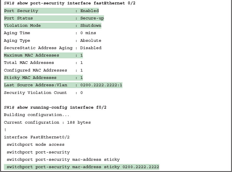
Example 8: Using Port Security to Define Correct MAC Addresses of Particular Interfaces
The first two commands in Example 8 confirm that a security violation has occurred on FastEthernet 0/1, but no violations have occurred on FastEthernet 0/2. The show port-security interface fastethernet 0/1 command shows that the interface is in a secure-shutdown state, which means that the interface has been disabled because of port security. In this case, another device connected to port F0/1, sending a frame with a source MAC address other than 0200.1111.1111, is causing a violation. However, port Fa0/2, which used sticky learning, simply learned the MAC address used by Server 2.
The bottom of Example 8, as compared to the configuration in Example 7, shows the changes in the running-config because of sticky learning, with the switchport port-security mac-address sticky 0200.2222.2222 interface subcommand.
Port Security Violation Actions
Finally, the switch can be configured to use one of three actions when a violation occurs. All three options cause the switch to discard the offending frame, but some of the options make the switch take additional actions. The actions include the sending of syslog messages to the console, sending SNMP trap messages to the network management station, and disabling the interface. Table 1 lists the options of the switchport port-security violation {protect | restrict | shutdown} command and their meanings.

Table 1: Actions When Port Security Violation Occurs
Note that the shutdown option does not actually add the shutdown subcommand to the interface configuration. Instead, IOS puts the interface in an error disabled (err-disabled) state, which makes the switch stop all inbound and outbound frames. To recover from this state, someone must manually disable the interface with the shutdown interface command and then enable the interface with the no shutdown command.
Port Security MAC Addresses as Static and Secure but Not Dynamic
To complete this lesson, take a moment to think about Analyzing Ethernet LAN Switching’s discussions about switching, along with all those examples of output from the show mac address-table dynamic EXEC command.
Once a switch port has been configured with port security, the switch no longer considers MAC addresses associated with that port as being dynamic entries as listed with the show mac address-table dynamic EXEC command. Even if the MAC addresses are dynamically learned, once port security has been enabled, you need to use one of these options to see the MAC table entries associated with ports using port security:
- show mac address-table secure: Lists MAC addresses associated with ports that use port security
- show mac address-table static: Lists MAC addresses associated with ports that use port security, as well as any other statically defined MAC addresses
Example 9 proves the point. It shows two commands about interface F0/2 from the port security example shown in Figure 5 and Example 7. In that example, port security was configured on F0/2 with sticky learning, so from a literal sense, the switch learned a MAC address off that port (0200.2222.2222). However, the show mac address-table dynamic command does not list the address and port, because IOS considers that MAC table entry to be a static entry. The show mac address-table secure command does list the address and port.

Example 9: Using the secure Keyword to See MAC Table Entries When Using Port Security

Configuring Basic Switch Management
INTERNOLD NETWORKS CCNA LIVE WEBCLASS (INCLW)
Configuring Basic Switch Management
Contents
Configuring Basic Switch Management
The work related to what a networking device does can be broken into three broad categories.
The first and most obvious, called the data plane, is the work a switch does to forward frames generated by the devices connected to the switch. In other words, the data plane is the main purpose of the switch.
Second, the control plane refers to the configuration and processes that control and change the choices made by the switch’s data plane. The network engineer can control which interfaces are enabled and disabled, which ports run at which speeds, how Spanning Tree blocks some ports to prevent loops, and so on.
The third category, the management plane, is the topic of this chapter. The management plane deals with managing the device itself, rather than controlling what the device is doing.
In particular, this lesson looks at the most basic management features that can be configured in a Cisco switch.
The first section of the lesson works through the configuration of different kinds of login security. The second section shows how to configure IPv4 settings on a switch so it can be remotely managed.
The last (short) section then explains a few practical matters that can make your life in lab a little easier.
Securing the Switch CLI
By default, a Cisco Catalyst switch allows anyone to connect to the console port, access user mode, and then move on to enable and configuration modes without any kind of security.
That default makes sense, given that if you can get to the console port of the switch, you already have control over the switch physically.
However, everyone needs to operate switches remotely, and the first step in that process is to secure the switch so that only the appropriate users can access the switch command-line interface (CLI).
This first topic in the lesson examines how to configure login security for a Cisco Catalyst switch.
Securing the CLI includes protecting access to enable mode, because from enable mode, an attacker could reload the switch or change the configuration.
Protecting user mode is also important, because attackers can see the status of the switch, learn about the network, and find new ways to attack the network.
Note that all remote access and management protocols require that the switch IP configuration be completed and working.
A switch’s IPv4 configuration has nothing to do with how a Layer 2 switch forwards Ethernet frames (as discussed in the lesson, “Analyzing Ethernet LAN Switching”), but to Telnet and Secure Shell (SSH) to a switch, the switch needs to be configured with an IP address.
In particular, this section covers the following login security topics:
- Securing user mode and privileged mode with simple passwords
- Securing user mode access with local usernames
- Securing user mode access with external authentication servers
- Securing remote access with Secure Shell (SSH)
Securing User Mode and Privileged Mode with Simple Passwords
Although the default switch configuration allows a console user to move into user mode and then privileged mode with no passwords required, unsurprisingly, the default settings prevent Telnet and SSH users from even accessing user mode.
And while the defaults work well to prevent unwanted access when you first install the switch, you need to add some configuration to then be able to sit at your desk and log in to all the switches in the LAN. In addition, of course, you should not allow just anyone to log in and change the configuration, so some type of secure login should be used.
The first option most people learn to secure access to user mode, one best used in a lab rather than in production, is a simple shared password. This method uses a password only—with no username—with one password for console users and a different password for Telnet users.
Console users must supply the console password, as configured in console line configuration mode. Telnet users must supply the Telnet password, also called the vty password, so called because the configuration sits in vty line configuration mode. Figure 1 summarizes these options for using shared passwords from the perspective of the user logging into the switch.

Figure 1: Simple Password Security Concepts
NOTE: This section refers to several passwords as shared passwords. These passwords are shared in the sense that when a new worker comes to the company, others must tell them (share) what the password is. In other words, each user does not have a unique username/password to use, but rather, all the appropriate staff knows the passwords.
In addition, Cisco switches protect enable mode (also called privileged mode) with yet another shared password called the enable password.
From the perspective of the network engineer connecting to the CLI of the switch, once in user mode, the user types the enable EXEC command. This command prompts the user for this enable password; if the user types the correct password, IOS moves the user to enable mode.
Example 1 shows an example of the user experience of logging into a switch from the console when the shared console password and the enable password have both been set.
Note that before this example began, the user started their terminal emulator, physically connected their laptop to the console cable, and then pressed the return key to make the switch respond as shown at the top of the example.

Example 1: Configuring Basic Passwords and a Hostname
Note that the example shows the password text as if typed (hope and love), along with the enable command that moves the user from user mode to enable mode. In reality, the switch hides the passwords when typed, to prevent someone from reading over your shoulder to see the password.
To configure the shared passwords for the console, Telnet, and for enable mode, you need to configure several commands. However, the parameters of the commands can be pretty intuitive. Figure 2 shows the configuration of all three of these passwords.

Figure 2: Simple Password Security Configuration
The configuration for these three passwords does not require a lot of work. First, the console and vty password configuration sets the password based on the context: console mode for the console (line con 0), and vty line configuration mode for the Telnet password (line vty 0 15). Then inside console mode and vty mode, respectively, the two commands in each mode are:
- login: Tells IOS to enable the use of a simple shared password (with no username) on this line (console or vty), so that the switch asks the user for a password
- password password-value: Defines the actual password used on the console or vty
The configured enable password, shown on the right side of the figure, applies to all users, no matter whether they connect to user mode via the console, Telnet, or otherwise. The command to configure the enable password is a global configuration command: enable secret password-value.
NOTE: Older IOS versions used the command enable password password-value to set the enable password, and that command still exists in IOS. However, the enable secret command is much more secure. In real networks, use enable secret. When we reach the devices security features lesson, we'll explain more about the security levels of various password mechanisms, including a comparison of the enable secret and enable password commands.
To help you follow the process, use the configuration checklist before the example.
The configuration checklist collects the required and optional steps to configure a feature. The configuration checklist for shared passwords for the console, Telnet, and enable passwords is:
- Step 1. Configure the enable password with the enable secret password-value command.
- Step 2. Configure the console password:
- A. Use the line con 0 command to enter console configuration mode.
- B. Use the login subcommand to enable console password security using a simple password.
- C. Use the password password-value subcommand to set the value of the console password.
- Step 3. Configure the Telnet (vty) password:
- A. Use the line vty 0 15 command to enter vty configuration mode for all 16 vty lines (numbered 0 through 15).
- B. Use the login subcommand to enable password security for vty sessions using a simple password.
- C. Use the password password-value subcommand to set the value of the vty password.
Example 2 shows the configuration process as noted in the configuration checklist, along with setting the enable secret password.
Note that the lines which begin with a ! are comment lines; they are there to guide you through the configuration.

Example 2: Configuring Basic Passwords
Example 3 shows the resulting configuration in the switch per the show running-config command. The gray lines highlight the new configuration. Note that many unrelated lines of output have been deleted from the output to keep focused on the password configuration.


Example 3: Resulting Running-Config File (Subset) Per Example 2 Configuration
Securing User Mode Access with Local Usernames and Passwords
Cisco switches support two other login security methods that both use per-user username/password pairs instead of a shared password with no username.
One method, referred to as local usernames and passwords, configures the username/password pairs locally—that is, in the switch’s configuration.
Switches support this local username/password option for the console, for Telnet, and even for SSH, but do not replace the enable password used to reach enable mode.
The configuration to migrate from using the simple shared passwords to instead use local usernames/passwords requires only some small configuration changes, as shown in Figure 3.

Figure 3: Configuring Switches to Use Local Username Login Authentication
Working through the configuration in the figure, first, the switch of course needs to know the list of username/password pairs. To create these, repeatedly use the username name secret password global configuration command.
Then, to enable this different type of console or Telnet security, simply enable this login security method with the login local line.
Basically, this command means “use the local list of usernames for login.”
You can also use the no password command (without even typing in the password) to clean up any remaining password subcommands from console or vty mode, because these commands are not needed when using local usernames and passwords.
The following checklist details the commands to configure local username login, mainly as a method for easier study and review:
- Step 1. Use the username name secret password global configuration command to add one or more username/password pairs on the local switch.
- Step 2. Configure the console to use locally configured username/password pairs:
- A. Use the line con 0 command to enter console configuration mode.
- B. Use the login local subcommand to enable the console to prompt for both username and password, checked versus the list of local usernames/passwords.
- C. (Optional) Use the no password subcommand to remove any existing simple shared passwords, just for good housekeeping of the configuration file.
- Step 3. Configure Telnet (vty) to use locally configured username/password pairs.
- A. Use the line vty 0 15 command to enter vty configuration mode for all 16 vty lines (numbered 0 through 15).
- B. Use the login local subcommand to enable the switch to prompt for both username and password for all inbound Telnet users, checked versus the list of local usernames/passwords.
- C. (Optional) Use the no password subcommand to remove any existing simple shared passwords, just for good housekeeping of the configuration file.
When a Telnet user connects to the switch configured as shown in Figure 3, the user will be prompted first for a username and then for a password, as shown in Example 4.
The username/password pair must be from the list of local usernames or the login is rejected.

Example 4: Telnet Login Process After Applying Configuration in Figure 3
NOTE: Example 4 does not show the password value as having been typed because Cisco switches do not display the typed password for security reasons.
NOTE: The username secret command has an older less-secure cousin, the username password command. Today, use the more secure username secret command.
Securing User Mode Access with External Authentication Servers
The end of Example 4 points out one of the many security improvements when requiring each user to log in with their own username. The end of the example shows the user entering configuration mode (configure terminal), and then immediately leaving (end). Note that when a user exits configuration mode, the switch generates a log message. If the user logged in with a username, the log message identifies that username; note the “wendell” in the log message.
However, using a username/password configured directly on the switch causes some administrative headaches. For instance, every switch and router needs the configuration for all users who might need to log in to the devices. Then, when any changes need to happen, like an occasional change to the passwords for good security practices, the configuration of all devices must be changed.
A better option would be to use tools like those used for many other IT login functions. Those tools allow for a central place to securely store all username/password pairs, with tools to make the user change their passwords regularly, tools to revoke users when they leave their current jobs, and so on.
Cisco switches allow exactly that option using an external server called an authentication, authorization, and accounting (AAA) server. These servers hold the usernames/passwords. Typically, these servers allow users to do self service and forced maintenance to their passwords. Many production networks use AAA servers for their switches and routers today.
The underlying login process requires some additional work on the part of the switch for each user login, but once set up, the username/password administration is much less. When using a AAA server for authentication, the switch (or router) simply sends a message to the AAA server asking whether the username and password are allowed, and the AAA server replies.
Figure 4 shows an example, with the user first supplying his username/password, the switch asking the AAA server, and the server replying to the switch stating that the username/password is valid.

Figure 4: Basic Authentication Process with an External AAA Server
While the figure shows the general idea, note that the information flows with a couple of different protocols. On the left, the connection between the user and the switch or router uses Telnet or SSH. On the right, the switch and AAA server typically use either the RADIUS or TACACS+ protocol, both of which encrypt the passwords as they traverse the network.
Securing Remote Access with Secure Shell
So far, this lesson has focused on the console and on Telnet, mostly ignoring SSH. Telnet has one serious disadvantage: all data in the Telnet session flows as clear text, including the password exchanges. So, anyone that can capture the messages between the user and the switch (in what is called a man-in-the-middle attack) can see the passwords. SSH encrypts all data transmitted between the SSH client and server, protecting the data and passwords.
SSH can use the same local login authentication method as Telnet, with the locally configured username and password. (SSH cannot rely on a password only.) So, the configuration to support local usernames for Telnet, as shown previously in Figure 3, also enables local username authentication for incoming SSH connections.
Figure 5 shows one example configuration of what is required to support SSH. The figure repeats the local username configuration as shown earlier in Figure 3, as used for Telnet.
Figure 5 shows three additional commands required to complete the configuration of SSH on the switch.

Figure 5: Adding SSH Configuration to Local Username Configuration
IOS uses the three SSH-specific configuration commands in the figure to create the SSH encryption keys. The SSH server uses the fully qualified domain name (FQDN) of the switch as input to create that key. The term FQDN combines the hostname of a host and its domain name, in this case the hostname and domain name of the switch.
Figure 5 begins by setting both values (just in case they are not already configured). Then the third command, the crypto key generate rsa command, generates the SSH encryption keys.
The configuration in Figure 5 relies on two default settings that the figure therefore conveniently ignored. IOS runs an SSH server by default. In addition, IOS allows SSH connections into the vty lines by default.
Seeing the configuration happen in configuration mode, step by step, can be particularly helpful with SSH configuration. Note in particular that in this example, the crypto key command prompts the user for the key modulus; you could also add the parameters modulus modulus-value to the end of the crypto key command to add this setting on the command.
Example 5 shows the commands in Figure 5 being configured, with the encryption key as the final step.


Example 5: SSH Configuration Process to Match Figure 5
Earlier, I mentioned that one useful default was that the switch defaults to support both SSH and Telnet on the vty lines. However, because Telnet is a security risk, you could disable Telnet to enforce a tighter security policy. (For that matter, you can disable SSH support and allow Telnet on the vty lines as well.)
To control which protocols a switch supports on its vty lines, use the transport input {all | none | telnet | ssh} vty subcommand in vty mode, with the following options:
- transport input all or transport input telnet ssh: Support both Telnet and SSH
- transport input none: Support neither
- transport input telnet: Support only Telnet
- transport input ssh: Support only SSH
To complete this section about SSH, the following configuration checklist details the steps for one method to configure a Cisco switch to support SSH using local usernames. (SSH support in IOS can be configured in several ways; this checklist shows one simple way to configure it.)
The process shown here ends with a comment to configure local username support on vty lines, as was discussed earlier in the section titled “Securing User Mode Access with Local Usernames and Passwords.”
- Step 1. Configure the switch to generate a matched public and private key pair to use for encryption:
- A. If not already configured, use the hostname name in global configuration mode to configure a hostname for this switch.
- B. If not already configured, use the ip domain-name name in global configuration mode to configure a domain name for the switch, completing the switch’s FQDN.
- C. Use the crypto key generate rsa command in global configuration mode (or the crypto key generate rsa modulus modulus-value command to avoid being prompted for the key modulus) to generate the keys. (Use at least a 768-bit key to support SSH version 2.)
- Step 2. (Optional) Use the ip ssh version 2 command in global configuration mode to override the default of supporting both versions 1 and 2, so that only SSHv2 connections are allowed.
- Step 3. (Optional) If not already configured with the setting you want, configure the vty lines to accept SSH and whether to also allow Telnet:
- A. Use the transport input ssh command in vty line configuration mode to allow SSH only.
- B. Use the transport input all command (default) or transport input telnet ssh command in vty line configuration mode to allow both SSH and Telnet.
- Step 4. Use various commands in vty line configuration mode to configure local username login authentication as discussed earlier in this chapter.
NOTE: Cisco routers default to transport input none, so that you must add the transport input line subcommand to enable Telnet and/or SSH into a router.
Two key commands give some information about the status of SSH on the switch. First, the show ip ssh command lists status information about the SSH server itself.
The show ssh command then lists information about each SSH client currently connected into the switch. Example 6 shows samples of each, with user Wendell currently connected to the switch.

Example 6: Displaying SSH Status
Enabling IPv4 for Remote Access
To allow Telnet or SSH access to the switch, and to allow other IP-based management protocols (for example, Simple Network Management Protocol, or SNMP) to function as intended, the switch needs an IP address, as well as a few other related settings. The IP address has nothing to do with how switches forward Ethernet frames; it simply exists to support overhead management traffic.
This next topic begins by explaining the IPv4 settings needed on a switch, followed by the configuration. Note that although switches can be configured with IPv6 addresses with commands similar to those shown in this chapter, this lesson focuses solely on IPv4. All references to IP in this lesson imply IPv4.
Host and Switch IP Settings
A switch needs the same kind of IP settings as a PC with a single Ethernet interface. For perspective, a PC has a CPU, with the operating system running on the CPU. It has an Ethernet network interface card (NIC). The OS configuration includes an IP address associated with the NIC, either configured or learned dynamically with DHCP.
A switch uses the same ideas, except that the switch needs to use a virtual NIC inside the switch. Like a PC, a switch has a real CPU, running an OS (called IOS). The switch obviously has lots of Ethernet ports, but instead of assigning its management IP address to any of those ports, the switch then uses a NIC-like concept called a switched virtual interface (SVI), or more commonly, a VLAN interface, that acts like the switch’s own NIC.
Then the settings on the switch look something like a host, with the switch configuration assigning IP settings, like an IP address, to this VLAN interface, as shown in Figure 6.

Figure 6: Switch Virtual Interface (SVI) Concept Inside a Switch
By using interface VLAN 1 for the IP configuration, the switch can then send and receive frames on any of the ports in VLAN 1. In a Cisco switch, by default, all ports are assigned to VLAN 1.
In most networks, switches configure many VLANs, so the network engineer has a choice of where to configure the IP address. That is, the management IP address does not have to be configured on the VLAN 1 interface (as configured with the interface vlan 1 command seen in Figure 6).
A Layer 2 Cisco LAN switch often uses a single VLAN interface at a time, although multiple VLAN interfaces can be configured. The switch only needs one IP address for management purposes. But you can configure VLAN interfaces and assign them IP addresses for any working VLAN.
For example, Figure 7 shows a Layer 2 switch with some physical ports in two different VLANs (VLANs 1 and 2).
The figure also shows the subnets used on those VLANs. The network engineer could choose to create a VLAN 1 interface, a VLAN 2 interface, or both. In most cases, the engineer plans which VLAN to use when managing a group of switches, and creates a VLAN interface for that VLAN only.

Figure 7: Choosing One VLAN on Which to Configure a Switch IP Address
Note that you should not try to use a VLAN interface for which there are no physical ports assigned to the same VLAN. If you do, the VLAN interface will not reach an up/up state, and the switch will not have the physical ability to communicate outside the switch.
NOTE: Some Cisco switches can be configured to act as either a Layer 2 switch or a Layer 3 switch. When acting as a Layer 2 switch, a switch forwards Ethernet frames as discussed in depth in the lesson, “Analyzing Ethernet LAN Switching.” Alternatively, a switch can also act as a multilayer switch or Layer 3 switch, which means the switch can do both Layer 2 switching and Layer 3 IP routing of IP packets, using the Layer 3 logic normally used by routers. This lesson assumes all switches are Layer 2 switches.
Configuring the IP address (and mask) on one VLAN interface allows the switch to send and receive IP packets with other hosts in a subnet that exists on that VLAN; however, the switch cannot communicate outside the local subnet without another configuration setting called the default gateway. The reason a switch needs a default gateway setting is the same reason that hosts need the same setting—because of how hosts think when sending IP packets. Specifically:
- To send IP packets to hosts in the same subnet, send them directly
- To send IP packets to hosts in a different subnet, send them to the local router; that is, the default gateway
Figure 8 shows the ideas. In this case, the switch (on the right) will use IP address 192.168.1.200 as configured on interface VLAN 1. However, to communicate with host A, on the far left of the figure, the switch must use Router R1 (the default gateway) to forward IP packets to host A. To make that work, the switch needs to configure a default gateway setting, pointing to Router R1’s IP address (192.168.1.1 in this case). Note that the switch and router both use the same mask, 255.255.255.0, which puts the addresses in the same subnet.

Figure 8: The Need for a Default Gateway
Configuring IPv4 on a Switch
A switch configures its IPv4 address and mask on this special NIC-like VLAN interface. The following steps list the commands used to configure IPv4 on a switch, assuming that the IP address is configured to be in VLAN 1, with Example 7 that follows showing an example configuration.
- Step 1. Use the interface vlan 1 command in global configuration mode to enter interface VLAN 1 configuration mode.
- Step 2. Use the ip address ip-address mask command in interface configuration mode to assign an IP address and mask.
- Step 3. Use the no shutdown command in interface configuration mode to enable the VLAN 1 interface if it is not already enabled.
- Step 4. Add the ip default-gateway ip-address command in global configuration mode to configure the default gateway.
- Step 5. (Optional) Add the ip name-server ip-address1 ip-address2 ... command in global configuration mode to configure the switch to use Domain Name System (DNS) to resolve names into their matching IP address.

Example 7: Switch Static IP Address Configuration
On a side note, this example shows a particularly important and common command: the [no] shutdown command. To administratively enable an interface on a switch, use the no shutdown interface subcommand; to disable an interface, use the shutdown interface subcommand.
This command can be used on the physical Ethernet interfaces that the switch uses to switch Ethernet messages in addition to the VLAN interface shown here in this example.
Also, pause long enough to look at the messages that appear just below the no shutdown command in Example 7. Those messages are syslog messages generated by the switch stating that the switch did indeed enable the interface. Switches (and routers) generate syslog messages in response to a variety of events, and by default, those messages appear at the console.
Configuring a Switch to Learn Its IP Address with DHCP
The switch can also use Dynamic Host Configuration Protocol (DHCP) to dynamically learn its IPv4 settings. Basically, all you have to do is tell the switch to use DHCP on the interface, and enable the interface. Assuming that DHCP works in this network, the switch will learn all its settings. The following list details the steps, again assuming the use of interface VLAN 1, with Example 8 that follows showing an example:
Step 1. Enter VLAN 1 configuration mode using the interface vlan 1 global configuration command, and enable the interface using the no shutdown command as necessary.
Step 2. Assign an IP address and mask using the ip address dhcp interface subcommand.

Example 8: Switch Dynamic IP Address Configuration with DHCP
Verifying IPv4 on a Switch
The switch IPv4 configuration can be checked in several places.
First, you can always look at the current configuration using the show running-config command.
Second, you can look at the IP address and mask information using the show interfaces vlan x command, which shows detailed status information about the VLAN interface in VLAN x.
Finally, if using DHCP, use the show dhcp lease command to see the (temporarily) leased IP address and other parameters. (Note that the switch does not store the DHCP-learned IP configuration in the running-config file.)
Example 9 shows sample output from these commands to match the configuration in Example 8.

Example 9: Verifying DHCP-Learned Information on a Switch
The output of the show interfaces vlan 1 command lists two very important details related to switch IP addressing.
First, this show command lists the interface status of the VLAN 1 interface—in this case, “up and up.” If the VLAN 1 interface is not up, the switch cannot use its IP address to send and receive management traffic. Notably, if you forget to issue the no shutdown command, the VLAN 1 interface remains in its default shutdown state and is listed as “administratively down” in the show command output.
Second, note that the output lists the interface’s IP address on the third line. If you statically configure the IP address, as in Example 7, the IP address will always be listed; however, if you use DHCP and DHCP fails, the show interfaces vlan x command will not list an IP address here. When DHCP works, you can see the IP address with the show interfaces vlan 1 command, but that output does not remind you whether the address is either statically configured or DHCP leased. So it does take a little extra effort to make sure you know whether the address is statically configured or DHCP-learned on the VLAN interface.
Miscellaneous Settings Useful in Lab
This last short section of the lesson touches on a couple of commands that can help you be a little more productive when practicing in a lab.
History Buffer Commands
When you enter commands from the CLI, the switch saves the last several commands in the history buffer. Then, as mentioned in Chapter 6, “Using the Command-Line Interface,” you can use the up-arrow key or press Ctrl+P to move back in the history buffer to retrieve a command you entered a few commands ago. This feature makes it very easy and fast to use a set of commands repeatedly. Table 1 lists some of the key commands related to the history buffer.

Table 1: Commands Related to the History Buffer
The logging synchronous, exec-timeout, and no ip domain-lookup Commands
These next three configuration commands have little in common, other than the fact that they can be useful settings to reduce your frustration when using the console of a switch or router.
The console automatically receives copies of all unsolicited syslog messages on a switch. The idea is that if the switch needs to tell the network administrator some important and possibly urgent information, the administrator might be at the console and might notice the message.
Unfortunately, IOS (by default) displays these syslog messages on the console’s screen at any time—including right in the middle of a command you are entering, or in the middle of the output of a show command. Having a bunch of text show up unexpectedly can be a bit annoying.
You could simply disable the feature that sends these messages to the console, and then re-enable the feature later, using the no logging console and logging console global commands. For example, when working from the console, if you want to temporarily not be bothered by log messages, you can disable the display of these messages with the no logging console global configuration command, and then when finished, enable them again.
However, IOS supplies a reasonable compromise, telling the switch to display syslog messages only at more convenient times, such as at the end of output from a show command. To do so, just configure the logging synchronous console line subcommand, which basically tells IOS to synchronize the syslog message display with the messages requested using show commands.
Another way to improve the user experience at the console is to control timeouts of the login session from the console or when using Telnet or SSH. By default, the switch automatically disconnects console and vty (Telnet and SSH) users after 5 minutes of inactivity. The exec-timeout minutes seconds line subcommand enables you to set the length of that inactivity timer. In lab (but not in production), you might want to use the special value of 0 minutes and 0 seconds meaning “never time out.”
Finally, IOS has an interesting combination of features that can make you wait for a minute or so when you mistype a command. First, IOS tries to use DNS name resolution on IP hostnames—a generally useful feature. If you mistype a command, however, IOS thinks you want to Telnet to a host by that name. With all default settings in the switch, the switch tries to resolve the hostname, cannot find a DNS server, and takes about a minute to timeout and give you control of the CLI again.
To avoid this problem, configure the no ip domain-lookup global configuration command, which disables IOS’s attempt to resolve the hostname into an IP address.
Example 10 collects all these commands into a single example, as a template for some good settings to add in a lab switch to make you more productive.

Example 10: Commands Often Used in Lab to Increase Productivity
